Sampling Approaches to Graph Clustering and Evaluation on the StringDB PPI

Supervised by Prof Georg Gottwald ~ Dec 2024

\(\newcommand{\Bf}[1]{\mathbf{#1}}\) \(\newcommand{\Bs}[1]{\boldsymbol{#1}}\)

Abstract

We introduce a new approach to performing community detection on networks. Our method involves creating many different partitions using the Louvain algorithm optimising over a sample of resolution parameters, and then iterating over the graph until we obtain consensus. We show that this method outperforms some other algorithms in benchmark graphs generated from the stochastic block model.

Table of Contents

1. Introduction
2. Methodology
   1. Sampling Resolutions
   2. Implementation
   3. Evaluation
   4. Bootstrapping
3. Results
   1. The MSE
   2. Hyperparameter Tuning
   3. Comparison to Other Methods
4. Limitations and Future Directions
5. Conclusion
6. References

Introduction

The StringDB Protein Protein Interaction (PPI) network is a graph with nodes representing the proteins in the Yeast strain Saccharomyces Cerevisiae (1). Edges between two nodes indicate a possible interaction link between the corresponding proteins. These links are estimated from a range of experimental and heuristic sources, so they may not represent a meaningful biological interaction. However, proteins tend to organise in higher-level structures like complexes and functional pathways. Such co-interaction may manifest in the StringDB PPI as a cluster of more densely connected nodes. These clusters may exist in many sizes and exhibit a high degree of mixing.

A common metric for determining whether a partition of an unweighted graph contains meaningfully dense clusters is modularity (2). Suppose we have a graph $G=(V,E)$ with adjacency matrix $A$, and denote the degree of node $i$ by $k_i$. Also, let $m$ be the total number of edges in the graph. Then the modularity for a partition $\mathbf C = (C_1,\dots, C_k)$ of $G$ is given by

Modularity weights the sum of observed links $A_{i,j}$ against the expected number of links between two nodes $i$,$j$ given their degrees. A good partition should have high modularity since the internal connectivity of a cluster would be much higher than expected.

A widely used method of partitioning a graph into communities is the Louvain algorithm. It is a greedy algorithm that attempts to maximise modularity. However, the Louvain algorithm suffers from two issues. Firstly, it is non-deterministic - even producing partitions with different numbers of clusters depending on a random initial seed (3). Secondly, modularity maximisation is insufficiently resolving on larger graphs, preferring to merge communities with fewer than $\sqrt{2m}$ edges - this shortfall is called the resolution limit (4).

A partial workaround to this resolution limit is offered by Reichardt and Bornholdt (5), who introduce a resolution parameter $\gamma > 0$ into the modularity equation

If $\gamma$ is large, then $A_{i,j} -\gamma \frac{k_i k_j}{2m} < 0$ for more pairs $i,j$ and hence the modularity is increased by cutting the edge between $i$ and $j$. In particular, modularity is maximised when the graph is partitioned into smaller clusters compared to that for standard modularity ($\gamma=1$). However, we observed that the Louvain algorithm’s output is highly sensitive to $\gamma$, and partitioning over a network by optimising over modularity with a fixed value of $\gamma$ would be unlikely to capture the entire range of true community sizes within in network.

An interesting question thus arises: is it possible to improve upon the Louvain algorithm by combining the partitions produced from different resolution parameters? It seems natural that the resulting partition would be more stable and incorporate more information about the structure of the graph. The situation recalls the concept of ensemble learning, where a diverse set of learning algorithms can better capture the complexity of the dataset and deliver better predictions than any individual algorithm.

In this report, we explore the ideas of Lancichinetti and Fortunato, who developed a framework for this type of ensemble clustering on graphs (3). Suppose we loosely consider a cluster as a subset of nodes with a higher intra-cluster edge density and a lower inter-cluster edge density than the rest of the graph. To perform ensemble learning with a family of clustering algorithms, Lancichinetti and Fortunato combine the partitions created by each algorithm to induce a transformation on the graph that increases intra-cluster edge density (increasing cluster cohesion) and reduces inter-cluster density (increasing cluster separation), making the graph easier to partition. Repeating this process many times would ideally split the graph into disconnected cliques which all the algorithms in the family would be able to correctly cluster, producing a consensus result.

To evaluate the performance of the consensus based approach, it would be ideal to have a set of true node cluster memberships to compare against, but there is no ground truth for complex networks like the StringDB PPI. Hence, we also ask: what alternative evaluation schemes exist when the ground truth is not known?

In this report, we explore a possible workaround by generating our own benchmark graphs using the stochastic block model, which takes a partition of nodes $\mathbf C =(C_1,\dots, C_k)$ and a symmetric matrix $P\in \mathbb R^{k \times k}$ where

and creates a random graph with clusters possessing these edge probabilities. We observed that sampling from stochastic block models with edge probabilities fitted to the StringDB PPI produced graphs with substantially similar characteristics to the PPI itself. We can then evaluate the performance of our consensus algorithm on these graphs since the cluster allocations of the stochastic block models are known. Drawing from the idea of the Bootstrap in statistics, these results would give us a reasonable estimate of the model’s classification accuracy on the StringDB PPI that is otherwise unavailable.

Methodology

For a graph $G=(V,E)$ with $n$ nodes, suppose we have a family of clustering algorithms $(L_j)_{j = {1,\dots, N}}$, where each $L_j : G \to \mathbf C$ is a clustering algorithm on the graph $G$ that produces some (possibly random) partition $\mathbf C = (C_1,C_2,\dots, C_k)$ of $G$.

Now, if we create $N$ partitions $(L_1(G), L_2(G),\dots, L_N(G))$ of $G$ using each clustering algorithm $L_j$ in our family, we can combine their results by representing their output as a matrix. Similarly to the group portfolio, let $R$ be the $n\times n$ matrix where

Lancichinetti and Fortunato refer to $R$ as the \textit{consensus matrix} (3). In particular, we can interpret $R$ as the weighted adjacency matrix of a weighted graph $G’$. This graph $G’$ will have more edges than $G$, since connections are formed any time two nodes are clustered together. Crucially, we can interpret the weight of an edge $(i,j)$ in $G’$ as the probability that the nodes $i$ and $j$ will be clustered together by an algorithm in the family $(L_j)_{j = {1,\dots, N}}$.

We expect edges with lower weights to connect nodes that lie between the boundaries of two or more clusters, where there is less likely to be consensus. Moreover, edges with higher weights would form between nodes that are connected in tightly bound communities.

To increase the separation between these clusters, we prune all edges in $G’$ below a threshold $\vartheta$. We can then apply our clustering algorithms $(L_{j})_{j \in {1,\dots,N}}$ to $G’$, and repeat these steps until the consensus matrix $R$ becomes block diagonal, and these blocks stop changing. We can interpret these diagonal blocks as our consensus partition.

The following algorithm summarises the Lancichinetti-Fortunato consensus method. Note that a limitation is that all the clustering algorithms in the family $(L_{j})_{j \in {1,\dots,N}}$ must be able to handle weighted graphs.

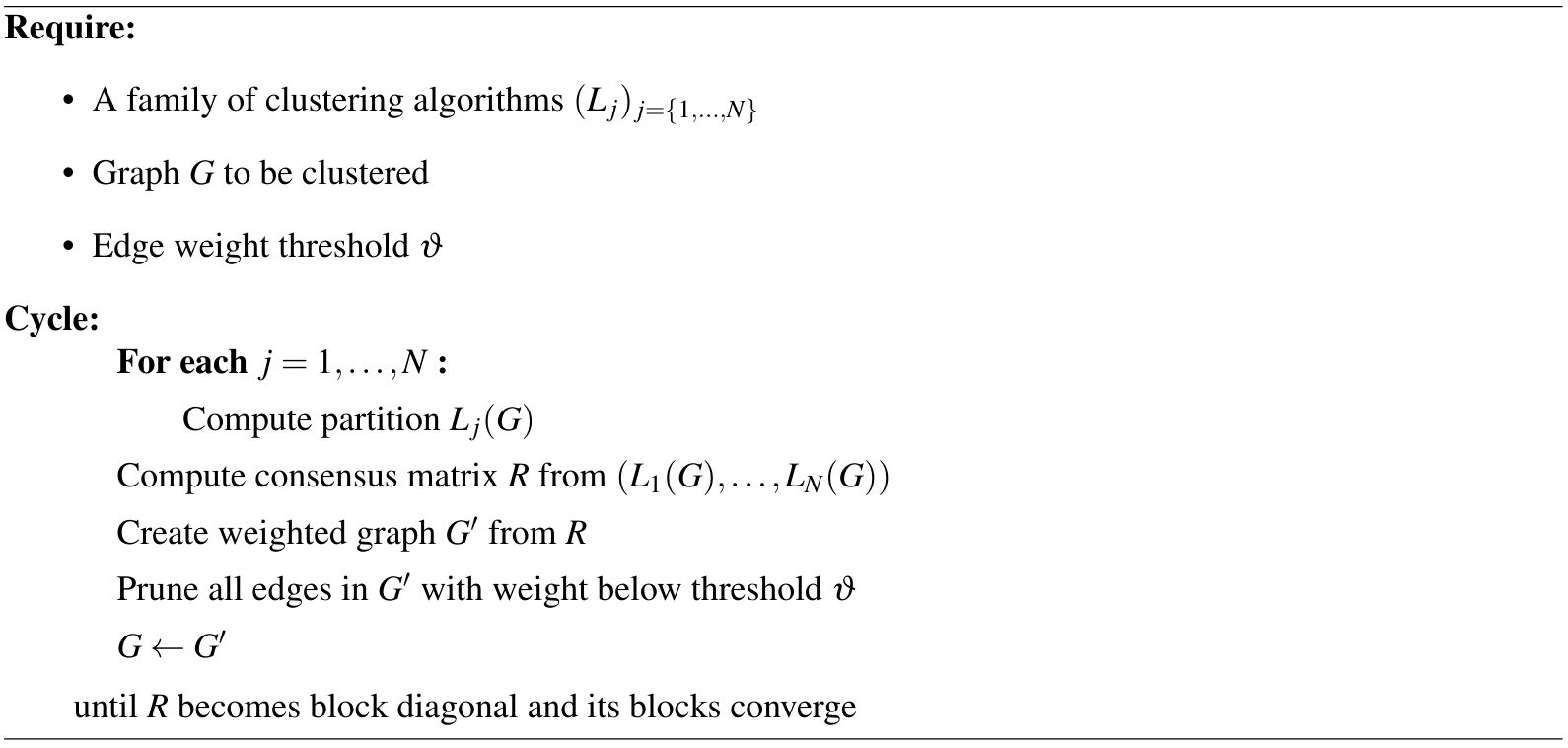
In the literature, there is only some heuristic discussion on why repeatedly applying this algorithm would force the diagonal blocks of $R$ to converge. We believe that any general result must assume some conditions on the clustering algorithms $(L_{j})_{j\in{1,\dots,N}}$ and their behaviour.

In particular, if we assume that the clustering algorithms will never assign two disconnected components to the same cluster, we can provide the following argument. Suppose that at some iteration of the algorithm, the consensus matrix $R$ has at least two blocks. The weighted network $G’$ built from $R$ must have a disconnected component for each block. By the assumption, nodes in a disconnected component cannot be clustered with nodes in another disconnected component for any clustering $L_i(G’)$. Hence, no pair of blocks in $R$ can join together in the updated consensus matrix created from the partitions $(L_i(G’))_{i\in{ 1,\dots, N}}$. Moreover, the thresholding step cannot merge two blocks either.

Therefore, each iteration can only increase the number of blocks in the consensus matrix, and nodes cannot change block membership. That is, if node $i$ is not in the same block with node $j$ at some iteration, then they will never be in the same block for any future iteration. Hence this loop must eventually halt – if the clustering algorithms cannot reach consensus, then the thresholding process will divide $R$ until it only contains diagonal blocks of size $1$.

In practice, for a graph with real clusters and reasonable algorithms that can detect them, $R$ does not get broken up into blocks of size $1$. The edge probabilities within each cluster will be pushed to $1$, and the repeated process ends up splitting the graph into cliques with high edge weights that are preserved through future iterations.

Sampling Resolutions

For a graph $G=(V,E)$ with $n$ nodes and $m$ edges, let $L_{\gamma}(G) = (C_1 ,\dots, C_{k})$ be the random partition representing the Louvain algorithm’s output on $G$ when maximising over modularity with resolution $\gamma$. To apply the consensus approach, we need a family of clustering algorithms. A natural choice is to create a family of Louvain algorithms, $(L_{\gamma_i})_{i\in {1,\dots, N}}$, each optimising over a unique $\gamma_i$ sampled from some distribution of resolutions.

To constrain this distribution, we follow the work of Jeub, Sporns and Fortunato (6) and define

i.e. the largest $\gamma$ such that applying the Louvain algorithm on $G$ with resolution $\gamma$ will return the whole graph as the singular cluster. Oppositely, let

i.e. the smallest $\gamma$ such that applying the Louvain algorithm on $G$ with resolution $\gamma$ will return each point as its singleton cluster. Resolution values outside of $[\gamma_{\min},\gamma_{\max}]$ are not interesting, so we restrict the density of $\gamma$ to take nonzero values only in this compact domain.

To compute $\gamma_{\max}$, we can take the minimum value $\gamma$ such that

for all $i,j$, so that the contribution of any cluster to the modularity is always negative. While there is no simple formula to compute $\gamma_{\min}$, we can approximate it by a simple binary search. We do not need to know $\gamma_{\min}$ very accurately, so we only compute it to two significant figures in our implementation.

It is known that ensemble methods perform better when the constituent algorithms are diverse. However, we observed that using equispaced points across $[\gamma_{\min}, \gamma_{\max}]$ did not yield good results. Often, $\gamma_{\max}$ would be a large value, so many sampled values of $\gamma$ were also large. The corresponding Louvain algorithms $L_{\gamma}$ would then create very fine partitions with too many clusters, making it difficult to achieve consensus. Hence, we want our sampling method to favour a region of the parameter space where the output of the clustering algorithm is still reasonable.

Ideally, the resolution $\gamma$ that we want our samples to concentrate around should be a value that allows the Louvain algorithm to generate sensible partitions. Fortunately, Newman (7) provides a rigorous framework for estimating the optimal resolution $\gamma_{\mathrm{opt}}$ for a graph. For our purposes, $\gamma_{\mathrm{opt}}$ is a natural choice for the resolution samples to concentrate around.

Newman’s idea was to show that optimising $\gamma$ is equivalent to fitting a network to a planted partition model and finding the maximum likelihood estimate of its parameters. If we suppose, for a graph $G$ and a fitted planted partition model with clustering $\mathbf C=(C_1,\dots,C_k)$ and parameters $(\omega_{\text{in}}, \omega_{\text{out}})$ where

and

then the log-likelihood estimate of the observed adjacency matrix $A$, given $\omega_{\text{in}}$ and $\omega_{\text{out}}$, is

where \(\omega_{i,j} = (\omega_{\text{in}} - \omega_{\text{out}})\unicode{x1D7D9}_{C_i,C_j} + \omega_{\text{out}}\)

is the probability of a connection between nodes $i$ and $j$ (7). If we also suppose that the probability of a connection between two nodes should be weighted by $k_ik_j/2m$, then the log-likelihood is instead

for some constants $\beta,\psi$ that are independent of our clustering $\mathbf C$, and

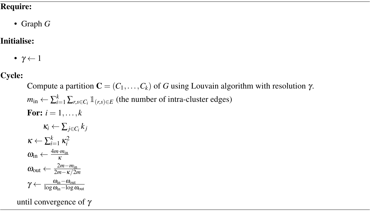
Hence, fitting a planted partition model to $G$ by maximising the log-likelihood is equivalent to finding the best resolution. The algorithm that Newman proposes to compute $\gamma_{\text{opt}}$ based on this equivalence is provided in Algorithm 2.

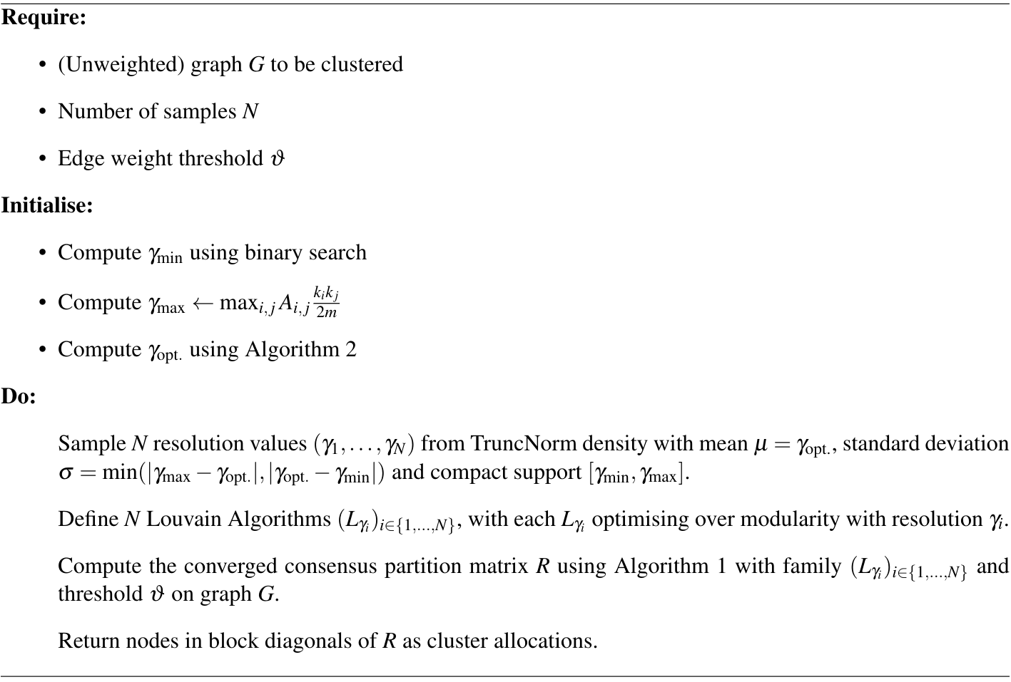
Therefore, we wish to sample from a density with compact support $[\gamma_{\min} ,\gamma_{\max}]$ and has greatest probability density at $\gamma_{\text{opt.}}$. In theory, there are many possible distributions, but for simplicity, we used the truncated normal centred at $\gamma_{\text{opt}}$. We found that a standard deviation of $\sigma = \min(|\gamma_{\max} - \gamma_{\mathrm{opt.}}| , |\gamma_{\mathrm{opt.}} - \gamma_{\min}|)$ provided a good balance between exploration and concentration around $\gamma_{\mathrm{opt.}}$.

Implementation

Recall that the Lancichinetti-Fortunato consensus approach requires clustering algorithms that can partition weighted graphs. Fortunately, there is a natural generalisation of the Louvain algorithm for weighted graphs (2). For a weighted graph $G = (V,E)$ with $n$ nodes and weighted adjacency matrix $A$ where

define the weighted degree of node $i$ by the sum of weights $w_i = \sum_{j=1}^n A_{i,j}$. Also, let $m$ be the sum of all edge weights in the graph. To generalise modularity for weighted graphs then, replace the node degrees $k_i$ in the original expression with the weighted node degrees $w_i$, to get

In this case, modularity is comparing the observed edge weight against the expected edge weight given the null model. The Louvain algorithm can simply optimise over this new modularity to partition a weighted graph. With this extension, we can finally perform consensus clustering as described in Algorithm 1, and the combined algorithm is described in Algorithm 3.

Our consensus algorithm is reasonably quick since it is based on repeatedly applying the Louvain algorithm, which is very fast with $O(n\log n)$ complexity, scaled by a constant factor $N$ for the number of resolution samples. While the rate of convergence for computing $\gamma_{\text{opt}}$ and the consensus matrix $D$ have not been studied rigorously in the literature, we observed both algorithms were able to converge to acceptable tolerances in only a few iterations.

Evaluation

Our approach has two hyperparameters: the number of clustering algorithms $N_{\mathrm{partitions}}$ per consensus and the threshold $\vartheta$ for the consensus matrix. However, it is not possible to tune these hyperparameters on the StringDB PPI in traditional ways, like performing cross-validation, since there is no ground truth labelling of the StringDB PPI’s nodes for us to compute the model’s clustering accuracy.

Despite this, we believe it is possible to estimate clustering accuracy by generating graphs with known clusters and substantially similar edge connection properties to the StringDB PPI, and computing model accuracy on these graphs instead.

For ease of biological interpretability and to manage computational requirements, we consider a subgraph of the StringDB PPI. From the original $6538$ proteins and $1412421$ interaction links, we perform the following:

1. Remove all essential proteins from the graph.
2. Prune all interaction links with edge weight less than $700$, and convert the graph to an unweighted one.
3. Remove all proteins without a human homologue.
4. Keep only proteins that are in the Endoplasmic Reticulum or the Nucleus.

These filtering steps leave us with $890$ proteins and $4836$ edges, about four times larger than what was considered in the Group Portfolio. Denote the filtered graph by $G_{\mathrm{PPI}}$.

Bootstrapping from the PPI

To constrain the problem, we consulted with the biologists, who told us that the most biologically meaningful clusters have a size of about $10$ to $15$ proteins. Using only this assumption, we propose a new way of estimating our model’s performance by taking ideas from the bootstrap.

First, we compute a range of resolutions $[\varphi_{\min}, \varphi_{\max}]$ where $\varphi_{\min}$ is the minimum resolution such that applying the Louvain algorithm on $G_{\mathrm{PPI}}$ produces a partition with mean cluster size $10$, and $\varphi_{\max}$ is the maximum resolution for mean cluster size $15$. We determined this range to be about $[6.7, 10.8]$. Next, we draw some number $M$ of resolution samples $(\gamma_1,\dots, \gamma_M)$ from a Uniform$(\varphi_{\min}, \varphi_{\max})$ distribution, and compute the Louvain partition at each resolution.

For such a partition, say $L_{\varphi_i}(G_{\mathrm{PPI}})$ with $k$ clusters $(C_1,\dots, C_k)$, we can compute the probability

and define the symmetric $k\times k$ matrix $P$ where $P_{r,s} = \omega_{r,s}$. This is enough to define a stochastic block model for each resolution $\gamma_i$, from which we can sample new graphs. We use a stochastic block model because it is better able to preserve the degree distribution of $G_{\mathrm{PPI}}$. Many benchmark graphs, like the Lancichinetti–Fortunato–Radicchi benchmark (8), assume a power law degree distribution which $G_{\mathrm{PPI}}$ does not have. The sampling procedure is summarised in Algorithm 4.

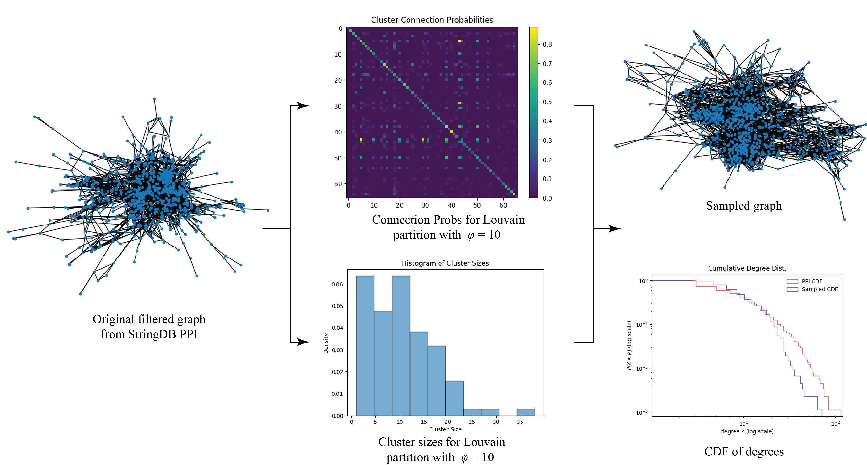
Figure 1 shows the process applied to one sample. The mean degrees of the graphs sampled from this process were very similar to the mean degree of $G_{\mathrm{PPI}}$, and the shapes of the CDFs were also very similar. However, we observed that our sampled graphs tended to under-represent the proportion of nodes with very high degrees. We attribute this behaviour to the fact that edges form between two nodes with a constant probability in a stochastic block model, which smooths out the degree distribution within each cluster and yields less pronounced hub proteins. While we did not have time, we believe that it may be possible to correct this under-representation by randomly adding edges in a rich-gets-richer scheme. Regardless, this deviation is not large and only affects highly connected hub proteins in each cluster, which we argue is not a big problem because these proteins would have probably been easy to cluster correctly to begin with.

We also note that the cluster memberships generated by the Louvain algorithm are most likely incorrect. However, if we assume that the true clusters within $G_{\mathrm{PPI}}$ indeed have a size of roughly $10$ to $15$ nodes, then because the Louvain clusters display similar inter-cluster and intra-cluster mixing probabilities to $G_{\mathrm{PPI}}$, the sampled graphs should still be good representatives. That is because it is unlikely for the true clusters of $G_{\mathrm{PPI}}$ to deviate significantly from the mixing probabilities used to generate the sampled graphs, since these probabilities were computed from $G_{\mathrm{PPI}}$ itself.

Results

The Mean Squared Error (MSE)

We define a metric for clustering accuracy. For a partition of graph $G=(V,E)$ with $n$ nodes, define the $n\times n$ matrix $Q$ where

Let $Q_{\mathrm{True}}$ be the true cluster allocations of the nodes in $G$ and $Q_{\mathrm{Pred}}$ be the cluster allocations produced by a community finding algorithm. We can define the mean squared error (MSE) by

where we use the Froebenius norm. The idea is that if a pair of nodes are partitioned into incorrect clusters compared to the truth, then $|Q_{\mathrm{True}_{i,j}} - Q_{\mathrm{Pred}_{i,j}}|^2 =1$, and the error will increase. An accurate clustering that matches well with the true allocations will minimise the MSE.

Hyperparameter Tuning Results

We observed that the performance of our consensus approach does not improve significantly with increasing the number of Louvain algorithms in each consensus $(N_{\mathrm{partitions}})$ beyond $60$ samples. This occurs across a range of tested threshold values – a plot of MSE performance against $N_{\mathrm{partition}}$ is provided in Figure 2.

To explore the effect of the number of Louvain algorithms per consensus on the MSE performance, we generated $200$ graphs using Algorithm $4$. Then, we computed the MSE of the consensus algorithm on each graph at the resolutions $\gamma = 0.15,0.5, 0.9$, and using $N = 5, 10, 20, \dots,150$ Louvain algorithms per consensus result. It is clear that the performance of the model stabilises with around $60$ samples.

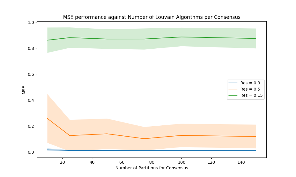
For this reason, we decided that taking $N_{\mathrm{partitions}} = 100$ is a good value that does not leave performance on the table.

Now, we draw a new sample of $200$ graphs. For each graph, we compute the MSE across a range of thresholds, taking the consensus of $N_{\mathrm{partitions}} = 100$ Louvain algorithms each time.

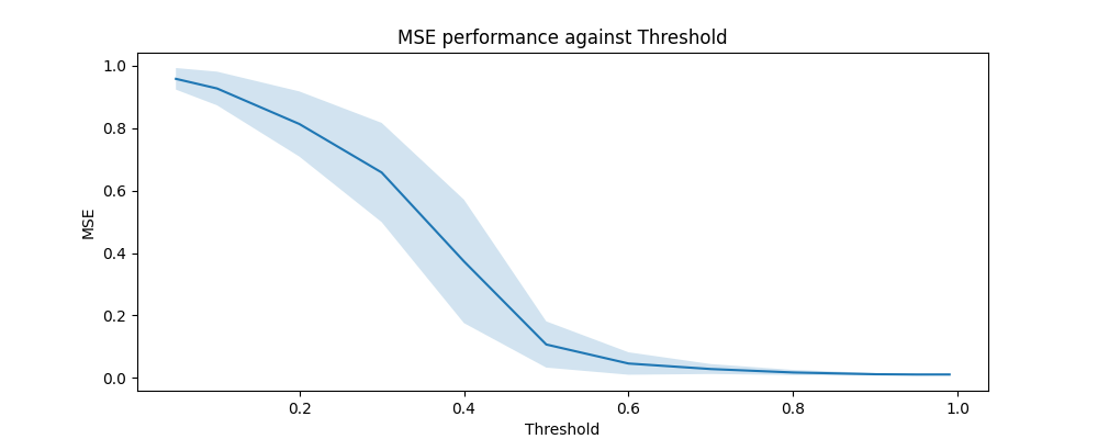
We observe a striking improvement in clustering accuracy performance as we increase the consensus threshold $\vartheta$ until about $\vartheta > 0.8$, where the MSEs stop decreasing. Moreover, as $\vartheta$ increases, the variance of the MSE values decreases – indicating that the consensus algorithm is producing more stable allocations.

Comparison to Other Methods

Now, we draw a sample of 200 graphs and partition each graph using some alternative algorithms. The results are shown in Figure 4

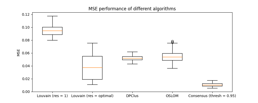
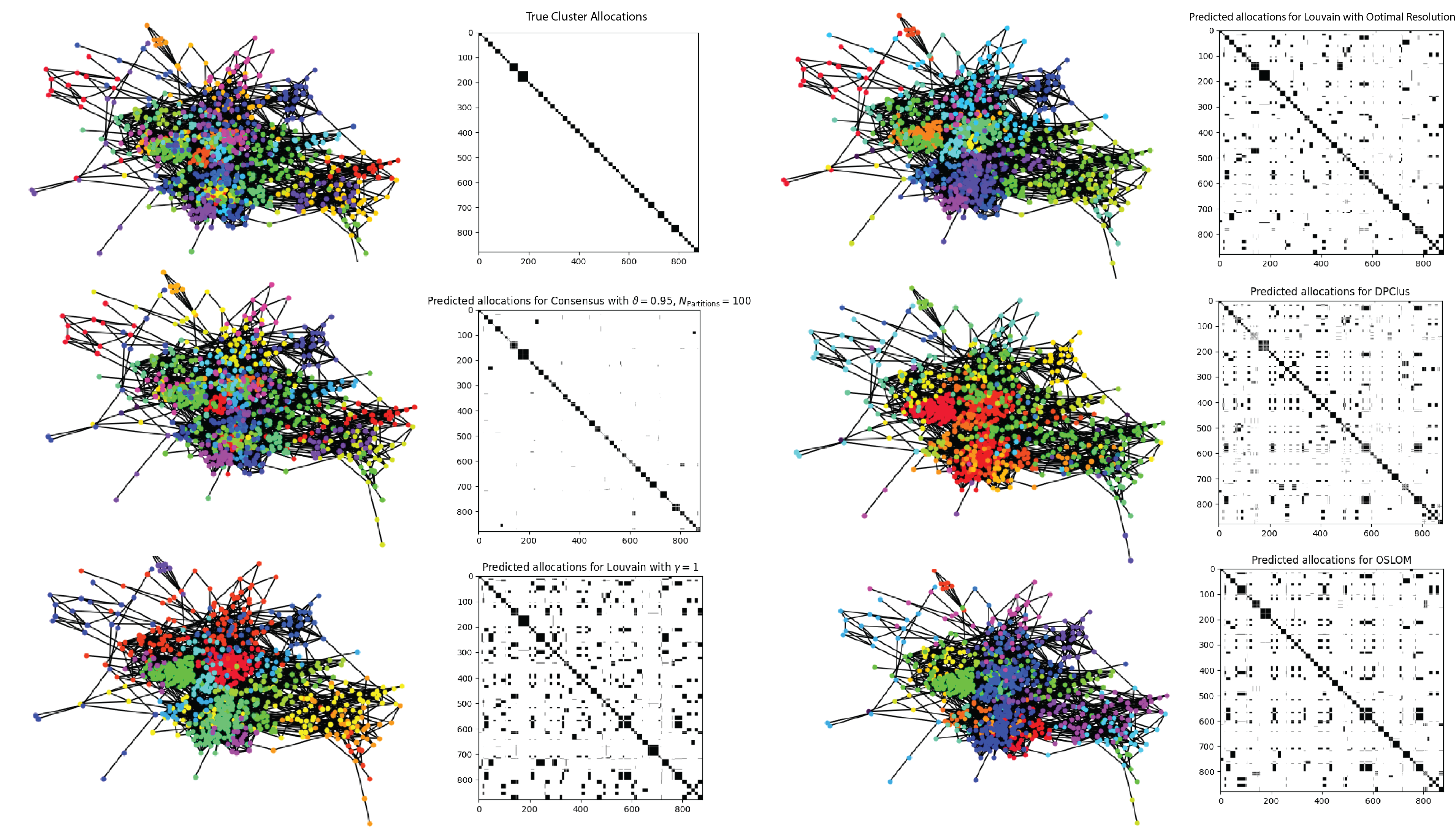
It is clear that the MSE performance of the consensus approach is significantly better than the other algorithms. The output of each clustering algorithm on the same graph is shown in Figure 5 and we can see from the pairwise allocation matrices that the consensus approach has the least noise.

Limitations and Future Directions

It is the case that in biological systems, proteins often play a part in many roles, and so proteins in the StringDB PPI may belong to many communities at once. Our approach is not able to identify this overlapping structure. However, there is work in the literature that explores alternative ways of using the consensus approach to identify these overlapping structures. Jeub, Sporns and Fortunato recently developed a method of fitting clusters produced from the Louvain algorithm at high resolutions inside of larger clusters that were produced at low resolutions to infer a hierarchical structure, revealing deeper organisation complexity (6). Another avenue of research could be to explore the consensus approach applied to different algorithms like OSLOM (9), DPClus (10), Infomap (11), and even spectral methods. Perhaps we may see an even greater improvement in MSE performance.

Conclusion

Our goal with this report was to explore ways of extending the Louvain algorithm by removing the need to specify a resolution parameter. To do this, we sampled from a range of resolution values, and created a family of Louvain algorithms, each optimising over modularity with their own resolution. We then used the consensus clustering framework of Lancichinetti and Fortunato to combine the partitions created by each algorithm in the family. We wanted to use this model to better detect clusters within networks with fuzzy and highly connected communities like the StringDB PPI. However, the true cluster allocations of each protein in the StringDB PPI are not known, so to evaluate the clustering accuracy of our model on the StringDB PPI, we developed a method of estimating this accuracy. Our idea was to fit a stochastic block model to the network, use the stochastic block model to generate graphs with similar cluster sizes and edge connectivity, and evaluate the mean squared error on these benchmark graphs instead.

Testing our approach on a filtered subgraph of the StringDB PPI, we found that our method produced considerable improvements in clustering accuracy compared to the Louvain algorithm with a fixed parameter – hinting that our method is unaffected by the resolution limit that plagues modularity maximisation algorithms. Our algorithm also outperforms OSLOM and DPClus. Finally, we identified some areas of future research, like exploring the consensus approach applied to different families of algorithms and adapting the consensus approach to identify hierarchy structures.

References

[1] Szklarczyk et al. The string database. Nucleic Acids Research, 51(10):638–646, 2023. doi: 10.1093/nar/gkac1000.

[2] M. E. J. Newman and M. Girvan. Finding and evaluating community structure in networks. Phys- ical Review E, 69(2), February 2004. ISSN 1550-2376. doi: 10.1103/physreve.69.026113. URL http://dx.doi.org/10.1103/PhysRevE.69.026113.

[3] Andrea Lancichinetti and Santo Fortunato. Consensus clustering in complex networks. Sci- entific Reports, 2(1), March 2012. ISSN 2045-2322. doi: 10.1038/srep00336. URL http://dx.doi.org/10.1038/srep00336.

[4] Santo Fortunato and Marc Barth´elemy. Resolution limit in community detection. Proceedings of the National Academy of Sciences, 104(1):36–41, 2007. doi: 10.1073/pnas.0605965104. URL https://www.pnas.org/doi/abs/10.1073/pnas.0605965104.

[5] Joerg Reichardt and Stefan Bornholdt. Detecting fuzzy community structures in complex networks with a potts model. Physical Review Letters, 93(21), 2004. doi: 10.1103/PhysRevLett.93.218701.

[6] Lucas G. S. Jeub, Olaf Sporns, and Santo Fortunato. Multiresolution consensus clustering in networks, 2018. URL https://arxiv.org/abs/1710.02249.

[7] M. E. J. Newman. Equivalence between modularity optimization and maximum likelihood methods for community detection. Physical Review E, 94(5), November 2016. ISSN 2470-0053. doi: 10.1103/phys- reve.94.052315. URL http://dx.doi.org/10.1103/PhysRevE.94.052315.

[8] Andrea Lancichinetti, Santo Fortunato, and Filippo Radicchi. Benchmark graphs for testing community detection algorithms. Physical Review E, 78(4), October 2008. ISSN 1550-2376. doi: 10.1103/phys- reve.78.046110. URL http://dx.doi.org/10.1103/PhysRevE.78.046110.

[9] Andrea Lancichinetti, Filippo Radicchi, Jos´e J. Ramasco, and Santo Fortunato. Finding statistically sig- nificant communities in networks. PLOS ONE, 6(4):1–18, 04 2011. doi: 10.1371/journal.pone.0018961. URL https://doi.org/10.1371/journal.pone.0018961.

[10] Hisashi Tsuji, Ken Kurokawa, Hiroko Asahi, Yoko Shinbo, and Shigehiko Kanaya. [special issue: Fact databases and freewares] dpclus: A density-periphery based graph clustering software mainly focused on detection of protein complexes in interaction networks. Journal of Computer Aided Chemistry, 7: 150–156, 09 2006. doi: 10.2751/jcac.7.150.

[11] Daniel Edler, Anton Holmgren, and Martin Rosvall. The MapEquation software package. https://mapequation.org, 2024.