Consistency Results on Estimating the Number of Clusters
Supervised by A/Prof Clara Grazian ~ Dec 2024
This is a short summary and introduction to the work. For the full project, see here.
Table of Contents
Background
To motivate the ideas behind this project, lets say that we are biologists, and we have collected some data about the heights of pea plants. Plotting our data in a histogram, we see this.
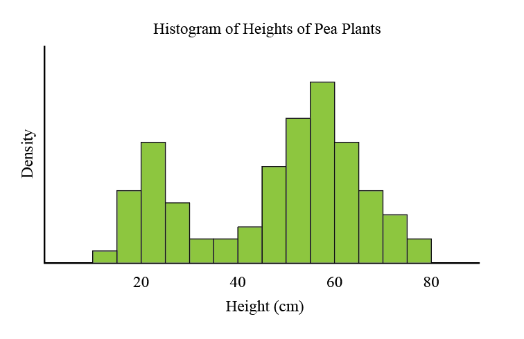
Clearly, our data cannot be modelled by a Normal distribution. It appears that roughly one quarter of pea plants belong to a cluster of shorter mean height, and the balance belonging to a cluster of taller plants. Indeed, this is expected, since the short gene was shown to be recessive by Mendel’s experiments with peas in the 1850s.
To model the heights of our pea plants then, it seems sensible to assume that the heights of each subpopulation (short plants and tall plants) are normally distributed, and superimpose these Normal distributions.
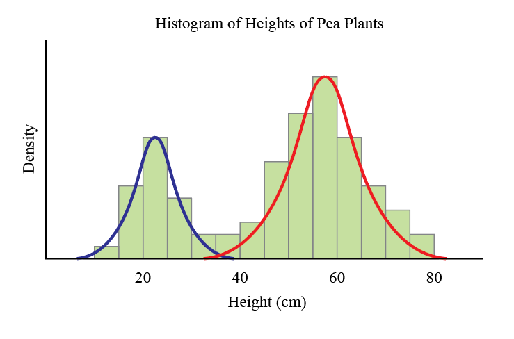
Of course, this idea can be generalised to any number of subpopulations and any type of distribution. We call these mixture models.
Definition (Mixture Model)
For some number of mixture components $t$; and distributions $R_j$ with weight $\pi_j$ for each $j=1,\dots, t$, the resulting mixture model has distribution \[ X_i\sim P = \sum_{j=1}^t \pi_j R_j\]
Mixture models are very flexible and can be used to make sense of many different types of data. However, there is a large drawback. Assuming we have a distribution in mind, in order to fit a mixture model to a dataset, we must specify the number of mixture components $t$ to fit.
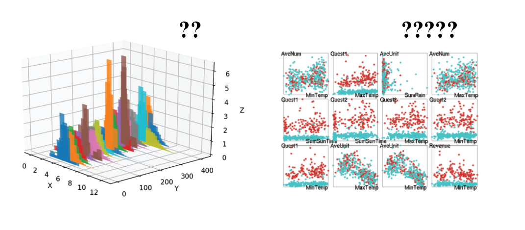
In the example of the pea plants, which is a one dimensional dataset, it is easy to see that there are most likely two mixture components. However, in higher dimensions, the picture is not always so clear.
Does that mean we simply choose the number of clusters that we want to see, and hope all is fine with our analysis?
No!
Fortunately, statisticians have developed many ways of estimating the number of mixture components. A popular method amongst Bayesians is to use a Dirichlet Process Mixture Model (DPMM) to simultaneously estimate the number of mixture components and fit a mixture model. Roughly, the idea is to create a mixture model with an infinite number of components, but at inference time, collapse the model so that only finitely many components have any mass.
To make sense of it all, we first introduce the Dirichlet distribution.
Definition (Dirichlet Distribution)
Let $Z_1,\dots, Z_k$ be independent random variables with $Z_j \sim \Gamma(\alpha_j,1)$. The Dirichlet distribution with parameter $(\alpha_1,\dots, \alpha_k)$, denoted $\mathrm{Dir}(\alpha_1,\dots,\alpha_k)$ is defined as the distribution of $(Y_1,\dots, Y_k)$ where \[ Y_j = \frac{Z_j}{\sum_{i=1}^{k} Z_i}\]
We can think of a draw from a Dirichlet distribution as a discrete probability distribution that is itself a random sample from a family of discrete probability distributions.
Now we define the Dirichlet process. It has two parameters, and we can think of it as a way to discretise a continuous distribution.
Definition (Dirichlet Process)
Denote $P\sim \mathrm{DP}(\alpha, Q_0)$ where
- $Q_0$ is the distribution from which we draw our probability distributions.
- $\alpha > 0$ controls the number of components.
Here are some simulated values with different values of $\alpha$ and $Q_0 \sim \mathrm{Normal}(0,1)$.
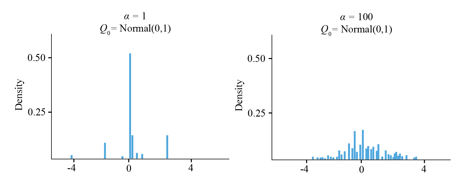
We see that when $\alpha$ is small, all of the mass of the base distribution becomes concentrated at a few points (the technical term is atom), and when $\alpha$ is large, there are many diffuse atoms, and the plot starts looking more like the base distribution. In particular, a draw from a Dirichlet Process is again a discrete probability distribution.
We can think of each atom as representing a mixture component, with the locations of each atom as a point in the parameter space, and the height of each atom as a mixture weight. In many ways then, we can view the Dirichlet process as a way of generating a random family of cluster distributions and weights. In the posterior, since there are finitely many atoms with nonzero mass, the Dirichlet process chooses the number of components in the mixture model implicitly.
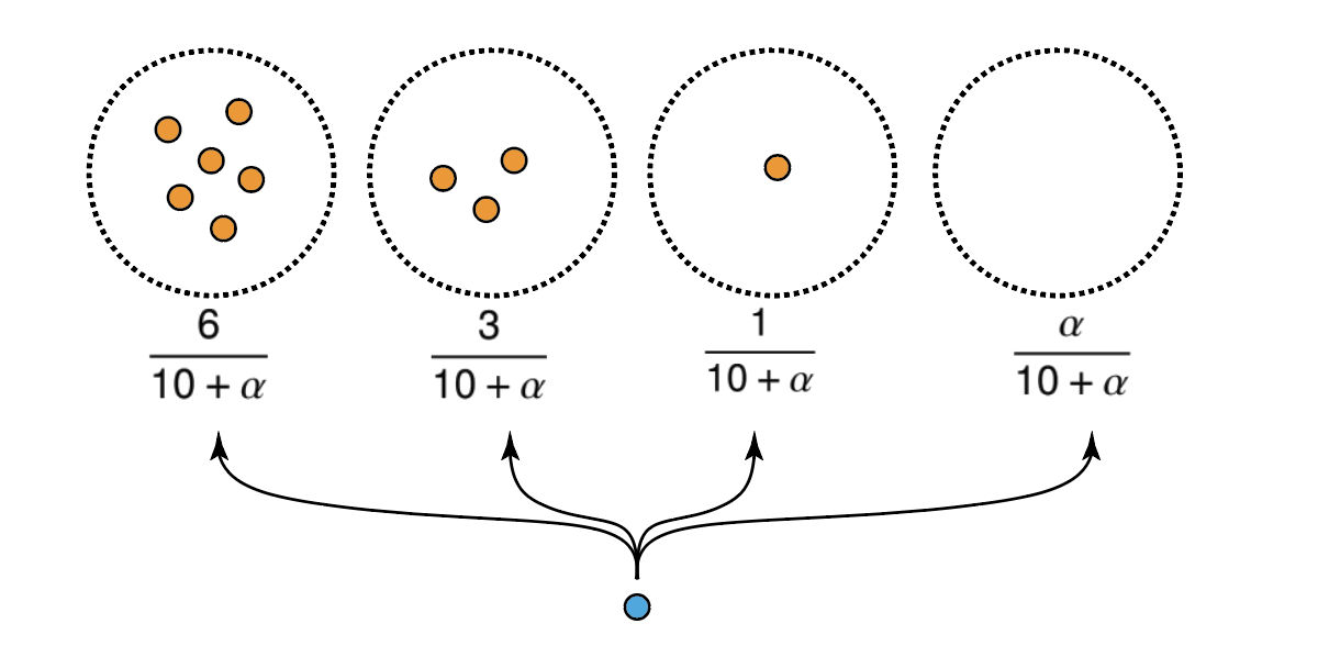
A useful property of the Dirichlet process is that clusters tend to be allocated according to a rich-gets-richer scheme, a result of the Bayes property of the Dirichlet distribution (Ferguson, 1973). In particular, for a sample $X_1,\dots, X_n$ generated from a Dirichlet process $\mathrm{DP}(\alpha,Q_0)$, if $c_k$ represents the component membership of $X_k$, and $\mathbf{c}_{-k}$ is the component memberships of all other observations, them
\[\mathbb{P}(c_k = i \mid \mathbf{c}_{-k} ,\alpha) = \frac{n_i}{n-1+\alpha} \,,\]where $n_i$ is the number of members in the $i$-th cluster, excluding possibly the $k$-th observation. Moreover, if there are $t$ components with data points, then the probability of an observation being sampled from a new component would be
\[1- \sum_{i=1}^t\mathbb{P}(c_k = i \mid \mathbf{c}_{-k} ,\alpha) = \frac{\alpha}{n-1+\alpha} \,.\]This behaviour is also called preferential attachment. Note that there is always a non-zero probability of a new cluster being made, though this probability decreases as the number of data points increases.
Finally we introduce the Dirichlet process mixture model:
Definition (Dirichlet Process Mixture Model)
For the following parameters,
- $P\sim\mathrm{DP}(\alpha,Q_0)$
- Cluster parameters $\theta_i\mid P\sim P$ for $i=1,2\dots$
Recall again that even though the Dirichlet process mixture model is an infinite sum, the mass is always at a finite number of components.
Now let’s explore how clustering and inference with a Dirichlet process mixture model works in practice.
Suppose we have data generated from a mixture of bivariate normal distributions, and we have already clustered the existing points into a blue and an orange cluster, and fitted bivariate normal distributions to each cluster. This is our prior information. Now say that we have just observed a new data point $X_k$.
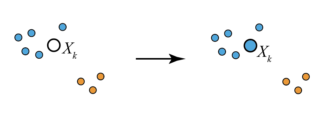
In practice, computing the posterior estimate for the component membership for $X_k$ involved computing the likelihood that the data was generated from each cluster weighted by the existing cluster size, with the best score winning out. In the case in Figure 6, we see that $X_k$ would be allocated to the blue cluster.
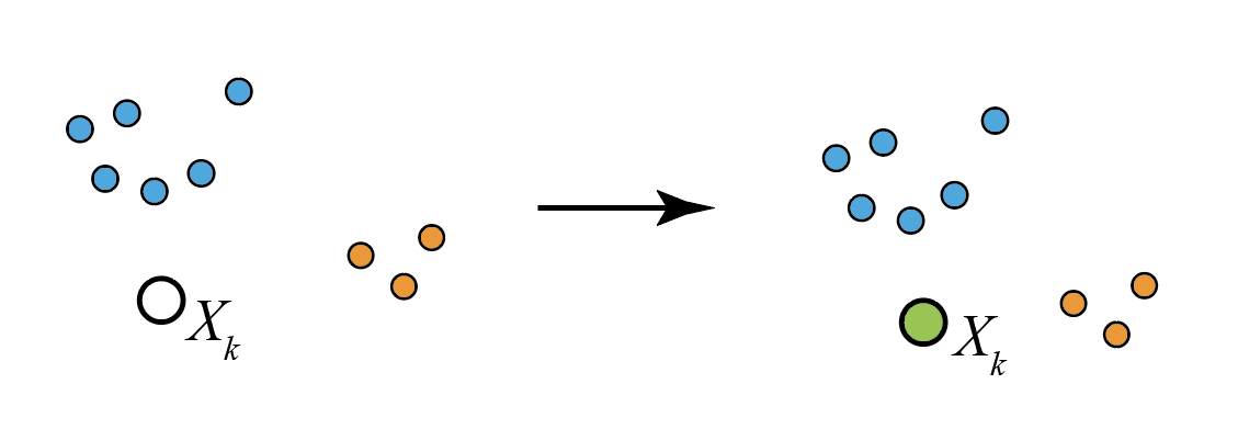
However, there is always the non-zero weight $\alpha/(n+\alpha)$ of being allocated to a new cluster, and fitting a new bivariate normal $N(\boldsymbol \mu, \Sigma)$ with $\boldsymbol \mu$ at the observed $X_k$ and the covariance matrix $\Sigma$ being some default value. In the case below, $X_k$ is very far from the blue and orange clusters, so the likelihood of being sampled from their distributions is low, even if the existing clusters are large. So the weight of creating a new cluster may win out, and $X_k$ is allocated to its own, green cluster.
Finally, we can introduce a generalisation of the Dirichlet process called the Pitman-Yor process. It provides more control over the cluster sizes, and has three parameters: a base distribution $Q_0$, a discount parameter $0\leq d<1$ and a concentration parameter $\alpha > -d$.
In a Pitman-Yor $\mathrm{PY}(\alpha, d, Q_0)$ process, the component membership probabilities instead satisfy
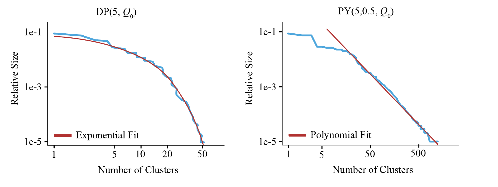
\[\mathbb{P}(c_k = i \mid \mathbf{c}_{-k} ,\alpha, d) = \frac{n_i- d}{n+\alpha} \quad \text{and} \quad 1- \sum_{i=1}^t\mathbb{P}(c_k = i \mid \mathbf{c}_{-k} ,\alpha) = \frac{td + \alpha}{n+\alpha} \,,\]In practice, this change means the expected cluster sizes of the Pitman-Yor model decreases with a power law relationship compared to an exponential decay with the Dirichlet process.
Questions
With this background out of the way, we ask a few questions.
Q1: As the number of data points $n\to\infty$, does the estimated number of clusters converge to the true value?
The answer to the first is No, if $\alpha, d$ are held constant (Miller and Harrison 2014)
Q2:Can we get consistency if $\alpha \mid \pi$ for some prior $\pi$?
Surprisingly, the answer is Yes, for Dirichlet processes.s (Ascolani et al. 2023)
Q3: Can we extend this to Pitman Yor Processes?
Maybe.
Literature Review
Miller and Harrison (2014)
Miller and Harrison (2014) were able to show that the Pitman-Yor process is not consistent for fixed parameters $\alpha,d$. Indeed, suppose the true number of clusters is $t$. Then their proof relies on proving three statements.
-
$\mathbb P (K_n = t + 1 \mid X_{1:n})$ is the same order of magnitude as $\mathbb P (K_n = t \mid X_{1:n})$, that is, the probability of overestimating the number of clusters is always large.
-
Let $A$ be a partition of $n$ data points into $t$ parts and $A’$ is a refinement into $t+1$ parts. We have $\mathbb P(X_{1:n} \mid A)$ has the same order of magnitude as $\mathbb P(X_{1:n} \mid A’)$, which encodes the idea that creating a new cluster to accommodate a point does not significantly lower the likelihood.
-
Under conditions 1 and 2, we have that the posterior estimate for the number of clusters is not consistent, and in particular.
Ascolani et al. (2023)
Ascolani et al. were able to show that estimating the number of clusters with the Dirichlet process mixture model with $\alpha\mid \pi$ is consistent. To do this, suppose the true number of clusters is $t$. Their proof relies on three main statements.
-
The ratio \(C(n,t,s) := \frac{\int \frac{\alpha^s \pi(\alpha)}{\alpha(\alpha+1)\cdots (\alpha+n-1)} d\alpha}{ \int \frac{\alpha^t \pi(\alpha)}{\alpha(\alpha+1)\cdots (\alpha+n-1)} d\alpha } \to 0 \text{ as } n\to\infty \,,\)
i.e. the addition of a prior $\pi$ favours a smaller number of clusters as $n\to\infty$.
-
The likelihood of the data being generated from $s$ clusters is bounded. \(R(n,t,s) := \frac{\sum_{A\in \tau_s(n)} \prod_{j=1}^s (|A_j|-1)!\prod_{j=1}^s m(X_{A_j}) }{ \sum_{B\in \tau_t(n)} \prod_{j=1}^t (|B_j|-1)!\prod_{j=1}^t m(X_{B_j}) } < \text{ ''grows slowly" }\)
-
Under 1 and 2, we have that
\[\lim_{n\to\infty}\mathbb P(K_n = t\mid X_{1:n}) = 1 \quad \text{ with probability } 1\,.\]that is, the estimator is indeed consistent.
Our Extension
In order to extend the results of Ascolani et al. from Dirichlet process models to Pitman Yor models, we need to replace the partition distribution of Dirichlet process
\[p(|A_1|,\dots,|A_k|) = \frac{\alpha^k}{(\alpha+1)_{n-1\uparrow 1}} \prod_{i=1}^k (|A_i|-1)! \,,\]with the partition distribution of the Pitman Yor process
\[p(|A_1|,\dots,|A_k|) = \frac{(\alpha+d )_{k-1\uparrow d}}{(\alpha+1)_{n-1\uparrow 1}} \prod_{i=1}^k(1-d)_{|A_i|-1 \uparrow 1} \,.\]and show that the same inequalities hold.
Indeed, we were able to show this result for the specific case of the Pitman-Yor process model where $\alpha\mid \pi$, $\pi \sim \mathrm{Uniform}(0,c)$ where $c$ is sufficiently small, and $d$ is a sufficiently small constant. We did this by extending the inequalities in Ascolani’s paper to cover the case of this prior.
It is important to note that for a Dirichlet process $\mathrm{DP}(\alpha, Q_0)$, the expected number of predicted clusters is $\mathbb E(K_n) \approx \alpha \log(n)$, and the goal of Ascolani et al. was to show that the addition of a prior modifies the behaviour of the model so that a new cluster is generated with less probability as the number of data points rises, cancelling out this logarithmic growth. However, for a Pitman-Yor process $\mathrm{PY}(\alpha, d, Q_0)$, the expected number of clusters $\mathbb E(K_n)$ is roughly $\alpha n^{d}$. This grows faster than the Dirichlet process, and hence, if we are to have any chance of producing the same consistency result, then it seems intuitive that we must have a very small discount parameter $d$.
Moreover, introducing a Uniform$(0,c)$ prior on $\alpha$ where $c$ is small means we are imposing a strong belief that the rate at which new clusters should be formed is small. This can be seen in the partition distribution of the Pitman-Yor process and also makes sense considering the growth rate of the clusters.