Hidden Markov Models for Analysing Stress Levels in Working Dogs
Supervised by A/Prof Clara Grazian ~ March 2024
For a summary of the project, see here.
For the original report as uploaded to AMSI, see here.
\(\newcommand{\Bf}[1]{\mathbf{#1}}\) \(\newcommand{\Bs}[1]{\boldsymbol{#1}}\)
Abstract
Working dogs are highly susceptible to heat stress because they engage in high-intensity activities, while they are bred to show resilience and ignore discomfort. We attempt to develop a quantitative model to predict the onset of heat stress in working dogs of the Kelpie breed using ECG, respiratory excursion, and temperature data collected from the dogs as they exercise throughout the day. We do this by fitting some hidden Markov models to the denoised data. We interpret the dogs’ underlying behavioural state by matching the estimated state sequence from the hidden Markov model with the activities the dogs engaged in at that time. We also evaluate the usefulness and tradeoffs of the different sensors for this analysis.
Table of Contents
Introduction
Motivation
Humans rely on working dogs for many tasks, including livestock herding, search and rescue services, and military missions. These tasks often demand high physical exertion over long durations and may also take place in high-temperature environments. As a result, dogs performing these tasks are at a high risk of temperature stress, which in serious cases, can become life-threatening.
In the field, handlers are responsible for assigning tasks to their working dogs (Thomas, 2022). Handlers also mandate rest periods to keep their dogs safe from overheating and heat stress. Handlers do this by observing behavioural cues: dogs experiencing heat stress will often pant heavily, seek shade and water, and exhibit an overall reluctance to move (Starling et al. 2022). However, using these behavioural cues for detecting heat stress in working dogs poses some challenges.
In particular, working dogs are specifically bred for resilience and to ignore discomfort, so they often do not show these warning signs until the dog is already heat-stressed (Starling et al. 2022). Moreover, some activities, like search and rescue, necessarily require the dog to work independently and potentially out of sight from their handlers. In these cases, handlers must plan out their dogs’ working and resting periods by estimating the rate at which their dogs’ internal body temperature will rise as a function of the type of activity they are doing and current environmental conditions (O’Brien et al. 2020). This estimation is made more challenging by the variation in fitness levels between different working dogs, meaning that the rate of body temperature increase in working dogs and their heat stress thresholds can vary considerably between different dogs and days. Crucially, the margin for error is small: while the typical body temperature for a working dog is $40.5-41^{\circ}\mathrm{C}$, the body temperature rising above $42^{\circ}\mathrm{C}$ can pose fatal dangers (Gordon, 2017).
To overcome the challenges of using qualitative behavioural cues, investigating methods of detecting heat stress in working dogs using quantitative analysis of sensor data would allow handlers to better protect the physical and mental well-being of the dogs they deploy.
Overview of Experiment
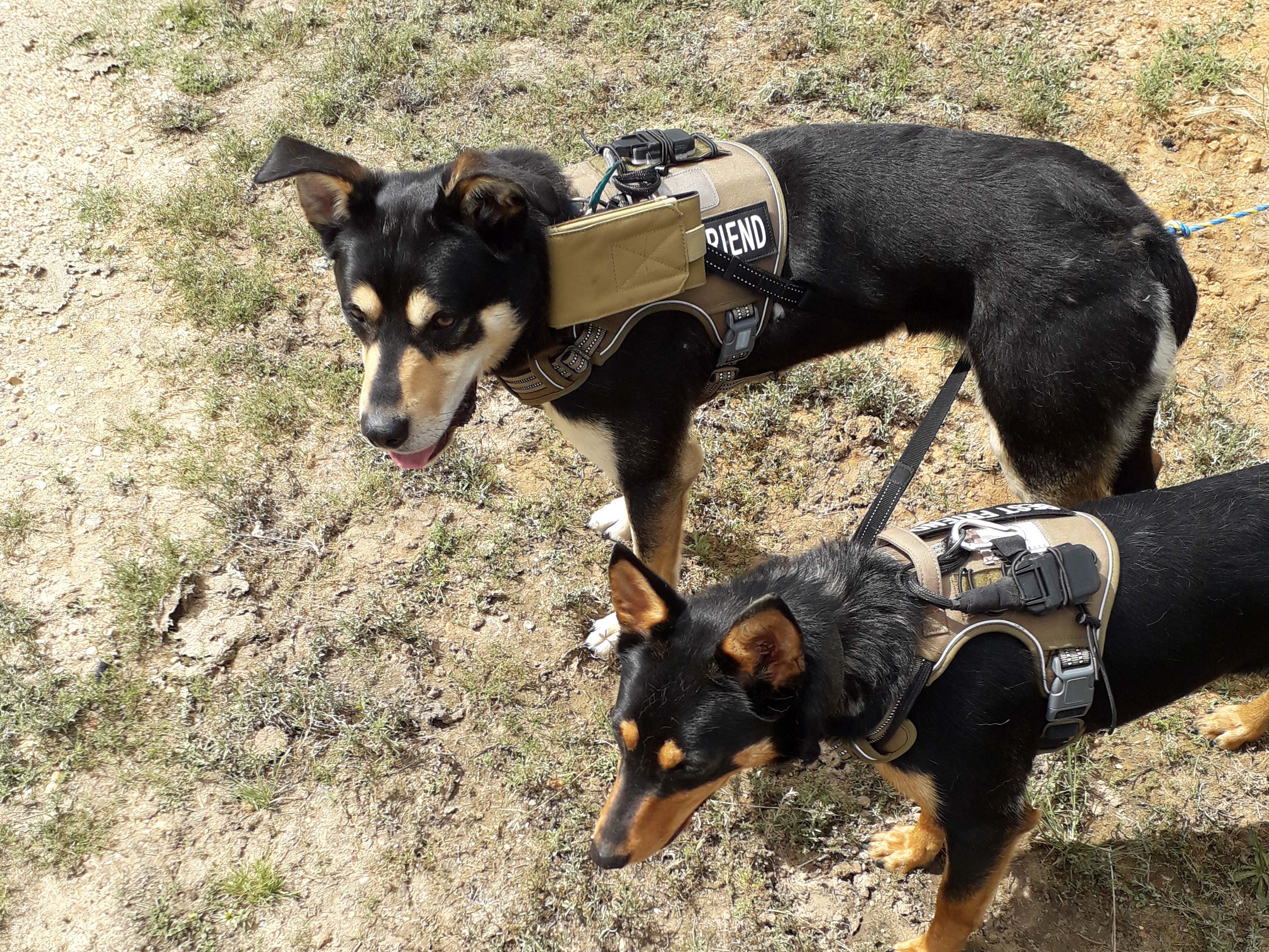
Starling et al. (2022) conducted an experiment over the summer of 2022 to collect data on working dogs for building a model for heat stress. Six working dogs of the Kelpie breed were fitted with a custom harness with sensors recording ECG, acceleration, respiratory excursions, and temperature data. Table 1 briefly describes how each data stream is collected.
| Data Stream | Brief Description of Sensor |
|---|---|
| ECG | Biopotential measurement performed by MAX30003 IC. Conductive gel applied to the ECG electrodes for better contact. |
| Respiratory Excursion | Constant current source through a piece of fabric (Holland Shielding) that changes resistance based on stretch. Voltage measured by the ADS1247 ADC. |
| Harness Temperature (Top/Bottom) | Temperature measurement performed by MAX30205 IC. |
| Internal Body Temperature | Measured by BodyCap temperature pill. Dogs administered pill 48 hours before experiment. |
| Integration | Harness supplied by Auroth Pets, microcontroller is the CC2640R2F. |
Table 1. Overview of data collection devices
The dogs also ingested a BodyCap pill which recorded their internal body temperature.
Throughout the day, the dogs engaged in four low-intensity exercises and one high-intensity exercise. All activities involved the dog following a chase vehicle (Starling et al. 2022). They are described below
Each exercise activity would be followed by a $1$ hour resting period. If a dog began lagging from the pace of the chase vehicle or exhibited a reluctance to move, the exercise would be halted, and the dog would be allowed to rest. This way, the dogs were always kept safe from heat stress.
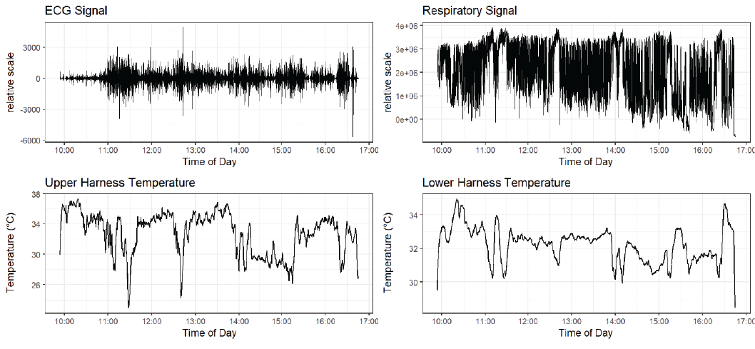
Data collected from the dog Bobby is shown in Figure 2.
HMMs for Animal Behaviour Analysis
To interpret the sensor data, we considered a biological model where the dog transitions between a group of underlying behavioural states, which can be interpreted as potential levels of stress. While we may not be able to observe the underlying behavioural state, for example, if the dog is experiencing a high level of potentially dangerous stress, we can always observe the sensor outputs which are assumed to be a direct result of the dog’s current behavioural state. We therefore wish to assign each of our recorded data points to these underlying behavioural states and use the activity timetable to identify states of stress.
This clustering process is most naturally represented by hidden Markov models (HMMs), which are a flexible family of models for the analysis and clustering of serially correlated time series data (Pohle et al. 2017). They have been successfully used to develop models for related biological problems like animal hunting movement (Mastrantonio et al. 2019) and whale diving behaviour (DeRuiter et al. 2017).
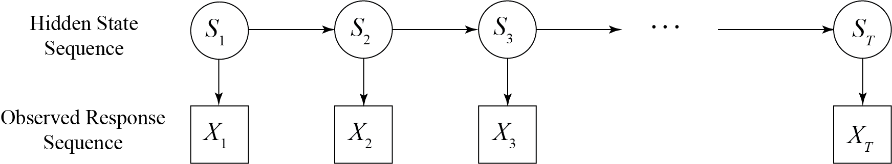
A hidden Markov model is defined by two sequences: a hidden state sequence, and an observed response sequence. Assuming that there are $N$ hidden behavioural states, we can model the activity state at time $t$ by the random variable $S_t$ with image points $S_t\in{1,2,\dotsb,N}$. We denote a state sequence of length $T$ by the random vector $S_{1:T} := (S_1,\dotsb,S_T)$, and we require the sequence to satisfy the Markov property, so for each $t = 2,\dotsb,T$ we have
\[ P(S_t \mid S_{1:(t-1)} ) = P(S_t\mid S_{t-1})\,. \]
We also represent the response sequence of length $T$ by a sequence of random variables $X_{1:T}=(X_1,\dotsb,X_T)$ where $X_t$ represents the measurement at time $t$. Importantly $X_t$ may be either a scalar or a random vector. We require, for each $t=1\dotsb,T$, the conditional dependence
\[ f(X_t\mid S_{1:t}, X_{1:{t-1}} ) = f(X_t\mid S_t) \,. \]
Figure 3 represents this conditional structure.
HMMs are therefore a natural way to analyse the working dog data because they automatically cluster each data point into underlying hidden states. For the data collected by the pill, let $X_{t,\mathrm{pill}}$ be the random variable modelling the internal body temperature at time $t$. For the data collected by the harness, let $\Bf{X}_{t, \mathrm{harness}}$ be a multivariate random variable modelling the ECG, respiratory excursion, and temperature observations at time $t$. Assume that $X_{t,\mathrm{pill}}$ can be modelled with a univariate Normal distribution, and $\Bf{X}_{t,\mathrm{harness}}$ with a multivariate Normal distribution.
Since the parameters of the normal distributions for $X_{t,\mathrm{pill}}$ and $\Bf{X}_{t,\mathrm{harness}}$ depend on the allocated level of stress for each data point, observations allocated to the same level of stress by the HMM are more likely to show similar values of temperature and other measurements, allowing us to make predictions about the stress level of the dog.
Aims
Our main aim for this report is to fit HMMs to the data collected by Starling et al. (2022). We aim to fit a univariate HMM to the pill data, and a multivariate HMM to the harness data. We then aim to use the clusters detected by these HMM models to interpret a \say{stressed} behavioural state and evaluate the use of HMMs for this application.
We also aim to test the quality of the data collected for this experiment and to understand whether we can interpret the level of stress of the dog only by looking at the recorded data and without knowing what the dog doing at the time.
Methodology
The experimental data also includes a complete list of the dogs’ activities and behaviours with corresponding observation times. However, we performed our analysis assuming that we did not know what the dog was doing and then interpreted our model with respect to the true activity sheet.
Overview of Data
The ECG and respiratory excursion sensors in the harness recorded data at a frequency of $100 \mathrm{Hz}$ and the temperature sensors at a frequency of $1 \mathrm{Hz}$. To fit HMMs to the data, we averaged every $100$ ECG and respiratory excursion observations to reduce their signal frequency to that of the temperature sensors. Since we are working with long time series, this shortening procedure was not a concern. However, in a future iteration of this experiment, it would be better to sample all the sensors at a common intermediate frequency like $10\mathrm{Hz}$.
Since the experiment relied on a custom-manufactured harness and sensor array, there were also some issues with the data collected. Table 2 summarises the issues found with each dog’s harness.
| Dog | Harness Faults |
|---|---|
| Abby | No data collected. |
| Bobby | No faults. |
| Franky | Respiratory excursion sensor disconnected after 2 hours. Harness temperature readings do not follow the same shape. |
| Toby | All data is present. Sometimes the values obtained by the harness sensors are erratic. Possibly a fit issue. Harness temperature readings do not follow the same shape. |
| Mallee | No data from temperature sensors on top and bottom of the harness. |
| Ruby | All data is present. Sometimes the values obtained by the harness sensors are erratic. Possibly a fit issue. |
Table 2. Overview of harness sensor faults afflicting each dog
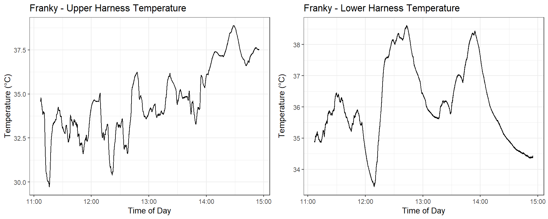
In the cases of Franky and Toby, the top and bottom temperature measurements from the dogs sometimes did not follow the same shape. Figure 4 shows this behaviour in Franky’s temperature sensors, where this discrepancy is very pronounced after 1:45 pm. We considered temperature data with this sort of divergence to be an inaccurate and invalid measurement of the dog’s true body temperature and did not use it in our analysis.
We also observed the BodyCap pill recording significant dips in internal body temperature when the dogs drank water. Figure 5 shows these dips in Bobby’s temperature pill graph.
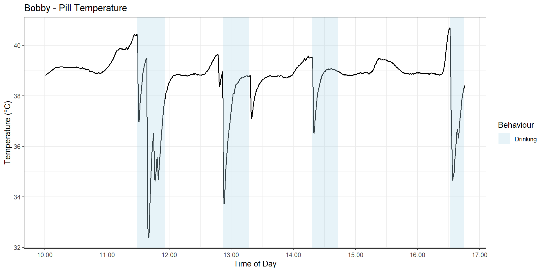
Throughout this report, we will focus mainly on the data cleaning and HMM analysis performed on the data collected by dog Bobby, since the data he generated was the most intact and free of errors. We will occasionally refer to other dogs when necessary.
Data Cleaning
The data collected is very noisy, with the largest contribution being the dog’s movements. The dog’s acceleration would directly induce noise into sensitive electronics like the ECG monitoring sensor. We could also observe the dog’s movement causing sporadic loss of contact between the sensors in the dog’s harness and their body. To deal with this, we applied some standard denoising steps to the data obtained from each sensor.
First, we perform initial data smoothing by applying a wavelet-based denoising method (Chatterjee et al. 2020). We used the denoise.dwt discrete wavelet denoiser from the rwt package (Roebuck 2014).
Next, we apply either a bandpass or lowpass Butterworth filter using the butter and filtfilt functions from the signal package (Ligges et al. 2023). The cutoff frequencies are described in Table 3.
| Data Stream | Corner Frequencies |
|---|---|
| ECG | Bandpass filter with corner frequencies 5Hz, 18Hz. These values were recommended by Jin et al. 2024 for preserving ECG features. |
| Respiratory Excursion | Lowpass filter with corner frequency 5Hz. This value was chosen empirically under the assumption that a dog does not pant at more than 300 breaths per minute (Becker 2011). |
| Harness Temperature (Top/Bottom) | Lowpass filter with corner frequency 8Hz. This value was chosen empirically. |
| Internal Body Temperature | Only the wavelet denoiser was applied. The data was considered sufficiently smooth and did not require further filtering. |
Table 3. Overview of filtering frequencies for each data stream
Parameter Estimation
To characterise the state sequence and response sequence of a hidden Markov model, we need to provide three sets of parameters. Assuming our HMM has length $T$ and there are $N$ hidden states, we can first decide upon an initial probabilities vector $\Bs{\theta}_{\mathrm{init.}} \in \mathbb{R}^N$ where the $i$-th coefficient is the probability $P(S_1=i)$ for $i\in {1,\dotsb, N}$, that is,
\[\Bs{\theta_{\mathrm{init.}}} = \begin{bmatrix} P(S_1 = 1) & \dotsb & P(S_1 = N) \end{bmatrix} \,.\]
We must also estimate the transition probabilities matrix $\Bs{\theta}_{\mathrm{trans.}} \in \mathbb{R}^{N\times N}$ where the $i,j$-th coefficient is given by
\[\Bs{\theta_{\mathrm{trans.}, i,j}} = P(S_t = i \mid S_{t-1} = j)\,\]
for $i,j\in {1,\dotsb,N}$. Moreover, for each possible state $S_t=i$, there is a conditional distribution for the response $X_t \mid S_t = i$. Under the assumption that the responses are normally distributed, we need to estimate $N$ pairs of mean and variance values, one pair for each state. Denote these estimated density parameters altogether as $\Bs{\theta}_{\mathrm{obs.}}$.
Having observed a sequence of responses $x_{1:T}$, we can estimate the parameters $\Bs{\theta_{\mathrm{init.}}}, \Bs{\theta_{\mathrm{trans.}}}$ and $\Bs{\theta_{\mathrm{obs.}}}$ (collectively $\Bs{\theta} := [ \Bs{\theta_{\mathrm{init.}}}, \Bs{\theta_{\mathrm{trans.}}}, \Bs{\theta_{\mathrm{obs.}}}]$), by maximising the likelihood function with respect to the parameter space, defined as
\[L(\Bs{\theta}|x_{1:T} ) = \sum_{i=1}^N f_{X_{1:T},S_T} (x_{1:T},S_T = i|\Bs{\theta}) \,.\]In the case of our experiment, this maximisation can only be done using numerical methods. Since the estimated transition matrix $\Bs{\theta_{\mathrm{trans.}}}$ must have columns that sum to $1$, and some of the parameters contained in $\Bs{\theta_{\mathrm{obs.}}}$ like the variance of each normal component must be positive, one may use either a general-purpose optimiser like BFGS-B, that can handle box constraints (Fletcher 1987), or apply a transformation to these variables so the overall optimisation problem becomes unconstrained (Zucchini, MacDonald & Langrock 2016). However, the HMM likelihood often contains many local maxima, hence real-world implementations involve running the optimisation algorithm over a large number of random starting points.
In the R language, which is an interpreted language with high overhead, attempting to perform direct maximisation on the likelihood function with multiple random starts proved to be too slow for the size of our dataset. To overcome this, we used an algorithm called expectation maximisation, which is a type of hill-climbing method that is empirically more resilient to local minima and is fast for Normal-distributed and Gamma-distributed responses. Our implementation of this algorithm, adapted from Visser & Speekenbrink (2022), is described in the Appendix.
The Viterbi Algorithm relies on two components. The first is a forward pass variable, denoted $\alpha_{t}(j)$ for $t = 1,\dotsb,T$ and $j = 1\dots, N$ where
\[\alpha_{t}(j) := \underset{s_{1:(t-1)}}{\mathrm{max}} f(S_{1:(t-1)} = s_{1:(t-1)}, S_t = j, x_{1:t}) \,,\]which keeps track of the joint density of the most likely state sequence ending at $S_t = j$ considering all the observations $x_1$ to $x_t$. Usefully, we can derive a recursive formula to calculate $\alpha$ quickly (Visser & Speekenbrink 2022), since
\[\begin{aligned} f(S_{t+1}, S_{1:t} , x_{t+1}, x_{1:t} ) &= f(x_{t+1}\mid S_{t+1}, x_{1:t}, S_{1:t}) P(S_{t+1}\mid x_{1:t}, S_{1:t})f(x_{1:t},S_{1:t}) \\ &= f(x_{t+1}\mid S_{t+1}) P(S_{t+1}\mid s_t)f(x_{1:t}, S_{1:t})\,. \end{aligned}\]which upon maximisation over all possible sequences $s_{1:t}$ yields
\[\alpha_{t+1}(i) = f(x_{t+1} \mid S_{t+1} =i) \cdot \underset{j} {\mathrm{max}} \ P(S_{t+1} = i \mid S_t =j)\alpha_{t}(j) \,.\]The second is a reverse pass variable, denoted $ \beta_{t}(i)$ for $t = 1,\dotsb,T$ and $i = 1\dots, N$ where
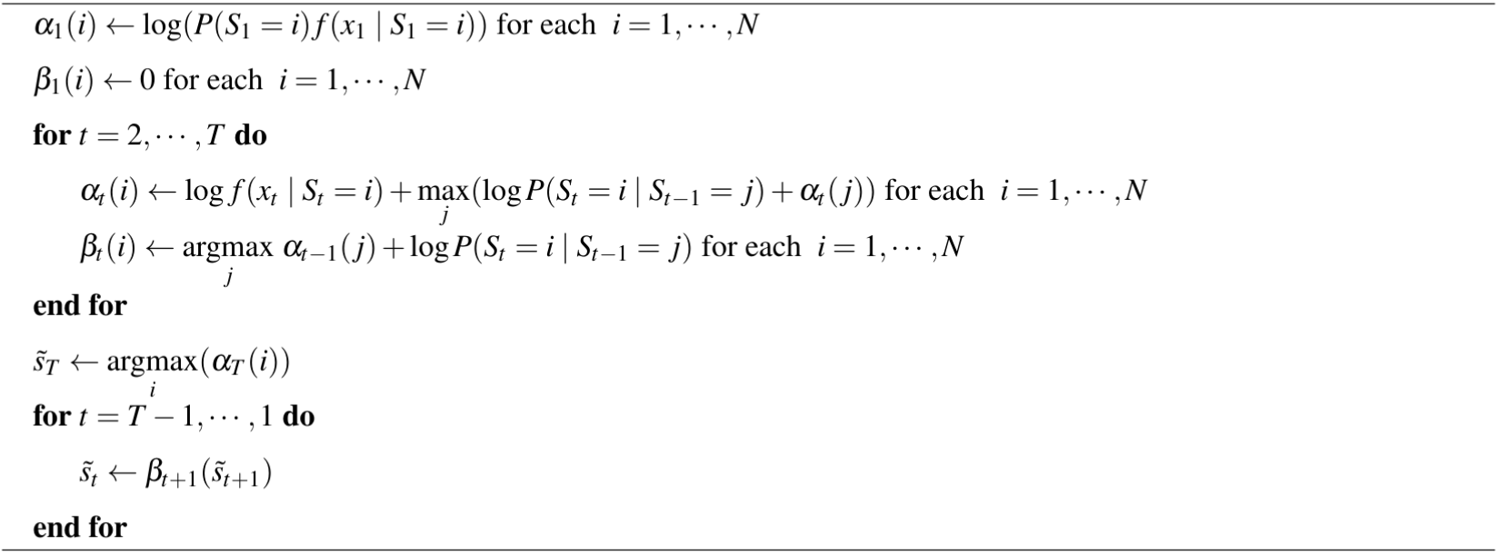
\[\beta_{t}(i) := \underset{j}{\mathrm{argmax}} \ \alpha_{t-1}(j) P(S_t = i\mid S_{t-1}=j) \,.\]The variable $\beta_{t}(i)$ tracks, for each state $S_t=i$, the most likely preceding state $S_{t-1}$. We implemented this algorithm by instead computing the log-densities and log-probabilities for better numerical behaviour, as shown in Algorithm 1.
Results
Model Selection
We were able to fit models of sizes $N=1,\dots,10$, while larger models exhibited numerical stability issues. The AIC/BIC scores for the univariate and multivariate models are plotted in Figure 6, showing that a global minimum point is not well defined in both cases.
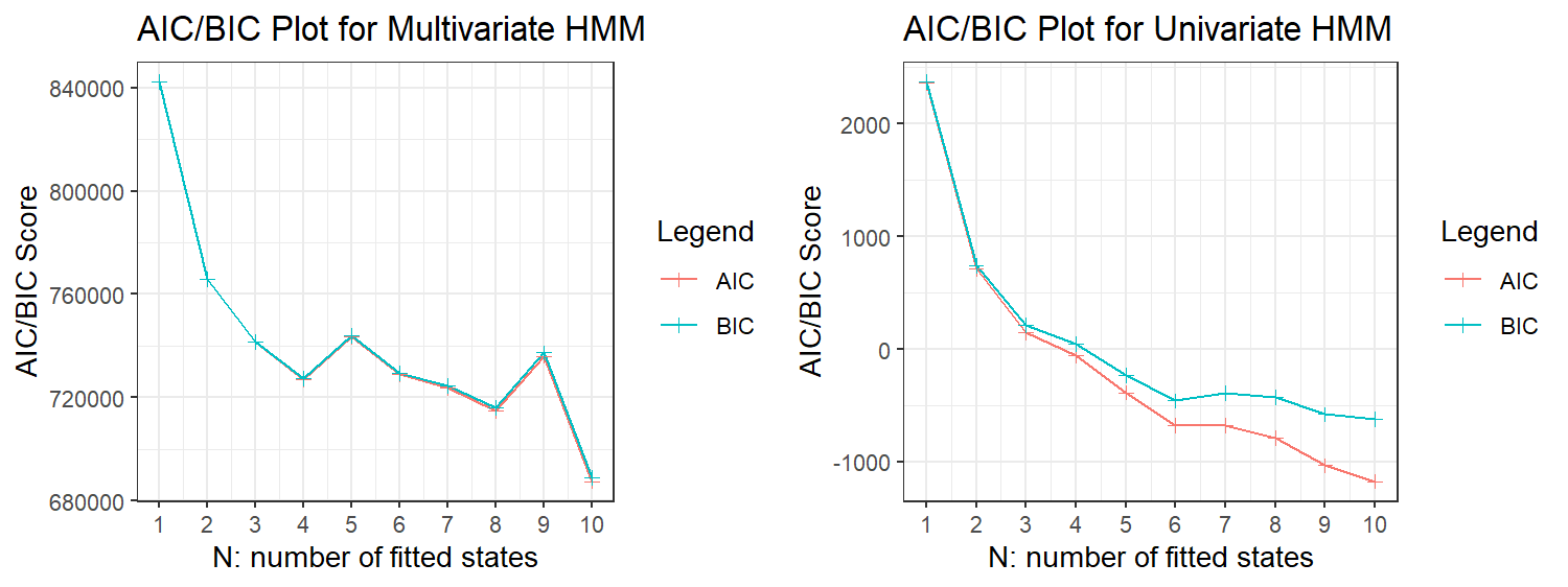
One possible reason is that the normal components we are using for our model response are only an approximation of the underlying data-generating process behind each observation (Pohle et al. 2017), leading the HMM to add extra states to account for this difference, even if these extra states do not have any biological meaning.
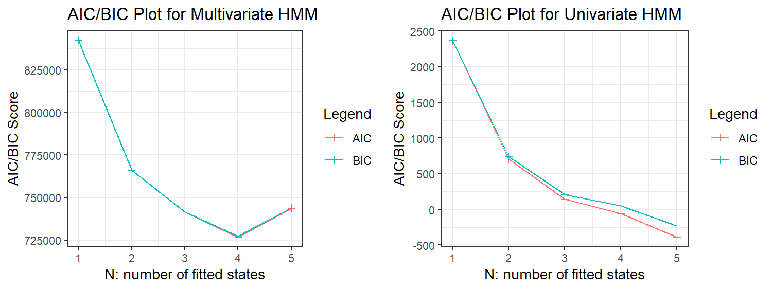
Recognising that AIC/BIC criteria tends to overestimate the number of hidden states, we decided that any model with more than $5$ hidden states was biologically implausible. Truncating our AIC/BIC plots at $5$ hidden states, as shown in Figure 7, we see that models with $3$, $4$ and $5$ hidden states have similarly low AIC and BIC scores, hence we considered them all as candidate models.
Univariate Pill Models
In this analysis, the colours are only used as labels and there is no correspondence with the colours between the $3$, $4$ and $5$ state models. Figure 8 shows the HMM fitted on Bobby’s pill data with three hidden states.
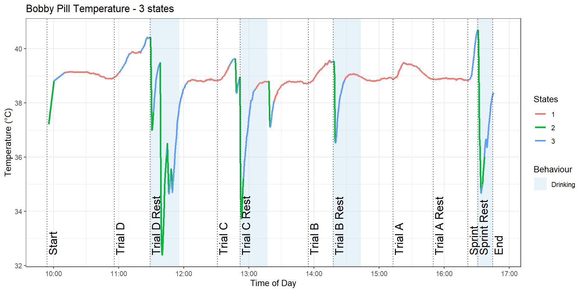
We can see that there is a low activity state in red that appears during the Trial $A$ and Trial $B$ activities, as well as the resting periods. The dog’s internal body temperature is stable during these times. We also see a higher-intensity exercise state in blue that appears during the sprint and parts of Trial $D$. Finally, we see that there is a green state that corresponds to sharp dips in temperature, caused by the dog drinking water.
With the addition of a fourth state, plotted in Figure 9, we see that the low activity state of the three-state model has split into a resting state, shown in green, and a low-intensity exercise state, in purple.
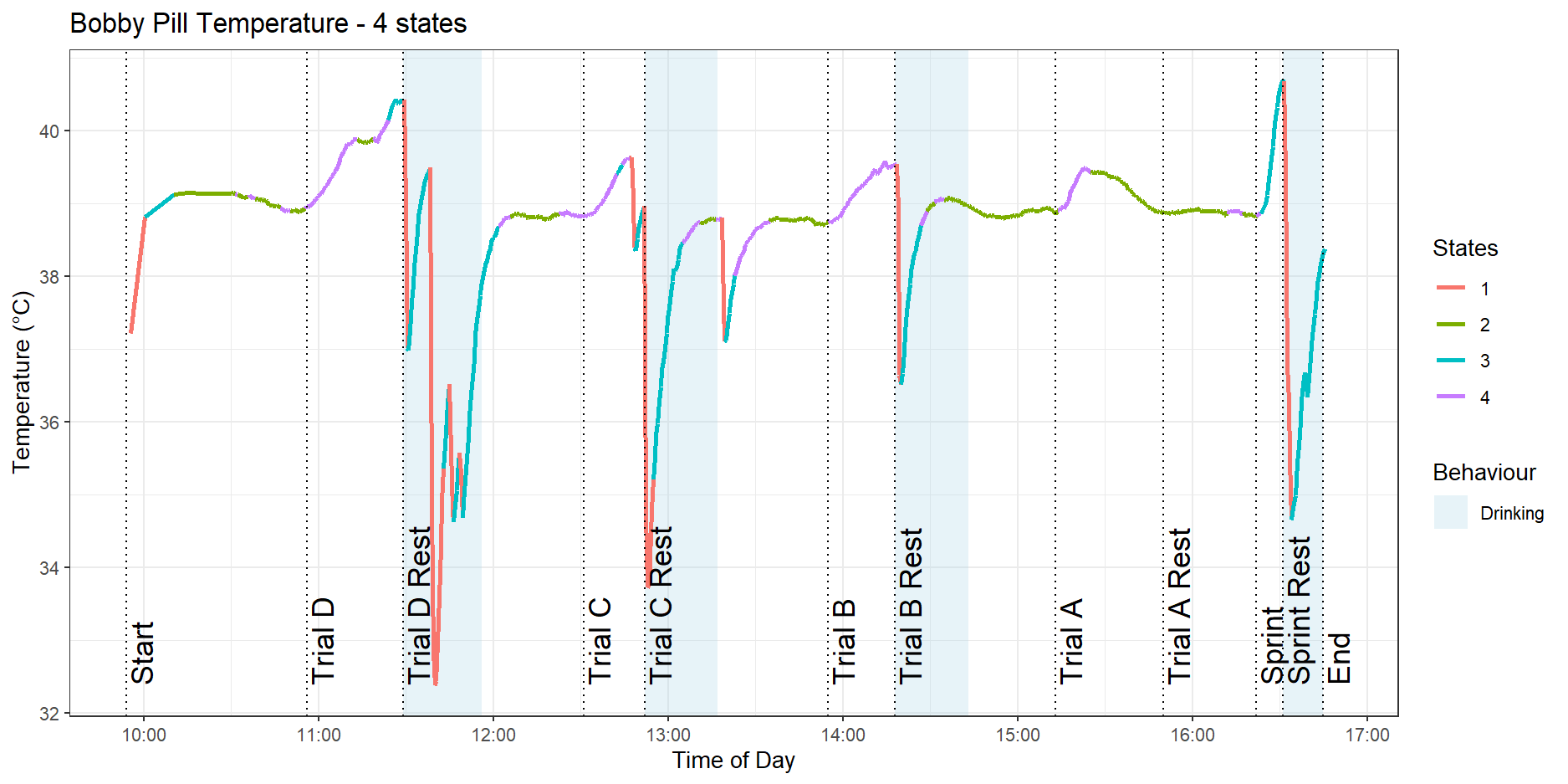
Usefully, the model can detect that the sprint is a higher-intensity activity and has clustered it in blue compared to the trot exercises in the purple state. However, we still see a red state allocated to sharp drops in temperature corresponding to the dog drinking water.
Adding the fifth state does not immediately yield a simple interpretation, as shown in Figure 10.
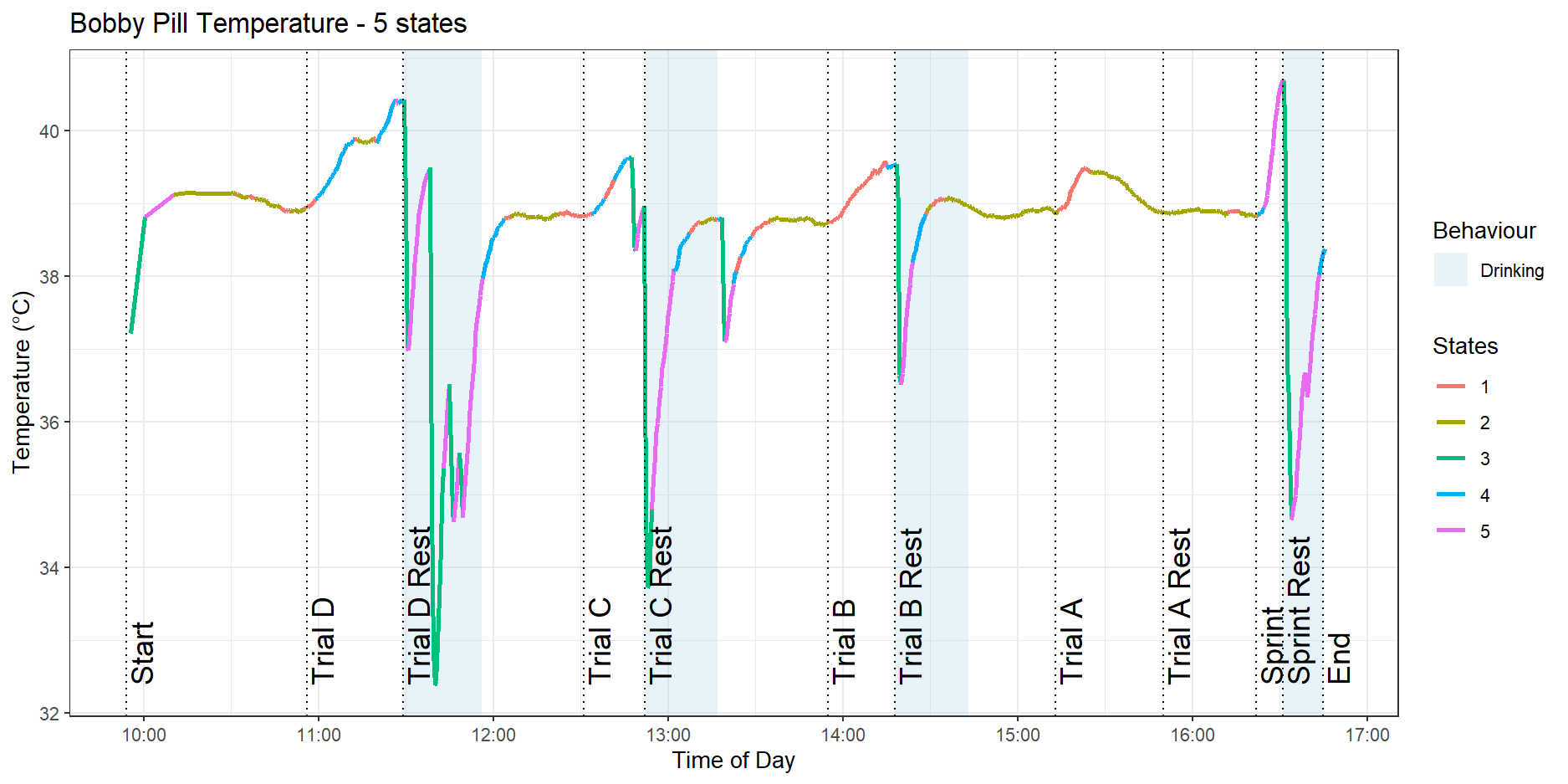
It is clear that the model is having trouble separating the sharp rises in temperature due to the dog drinking water from the dog performing high-intensity activities like the sprint exercise.
Multivariate Harness Models
The multivariate HMMs for the harness data were fitted using the depmixS4 package. The fitted three-state HMM for Bobby’s harness is shown in Figure 11.
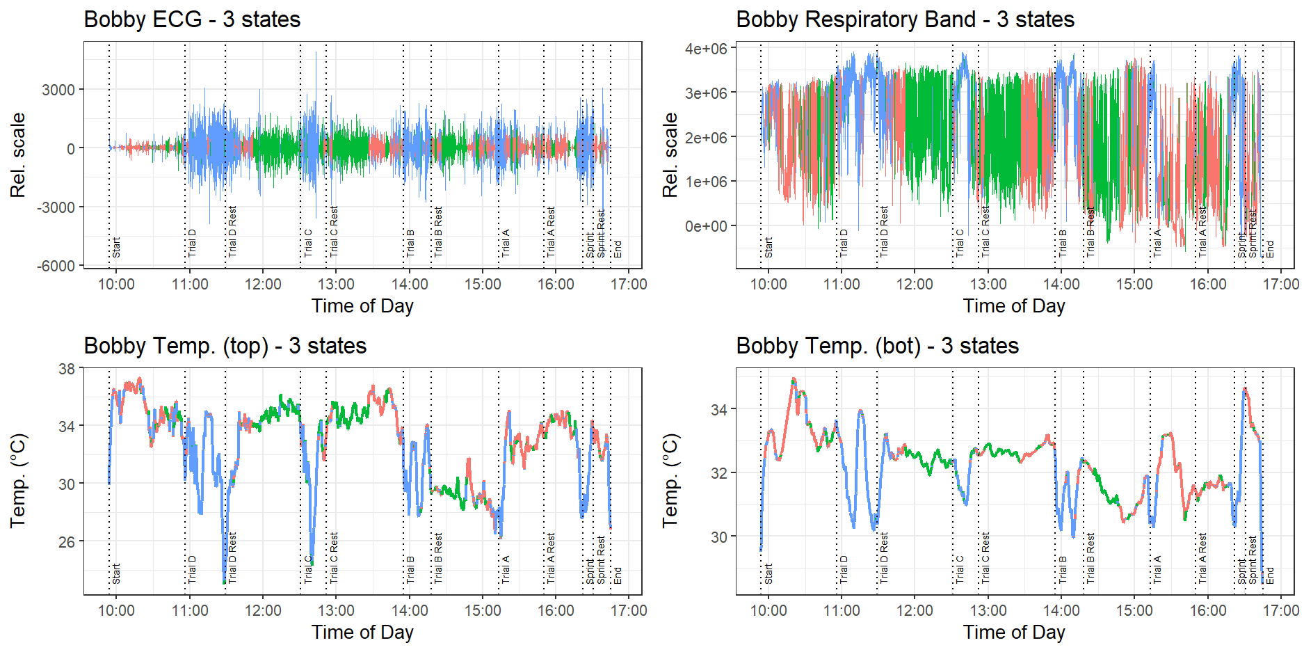
We see that the model can identify when the dog is exercising, and has clustered those points in blue. This is characterised by high variance in the recorded ECG and temperature signals, and higher mean in the respiratory band values. The model also divided the resting periods into a red and green state, with the red state characterised by lower magnitude ECG signals, and the green state by relatively stable temperature values. Reassuringly, the data collected by the harness does not seem to be affected by the dog drinking water. However, we still see some sharp dips in temperature, this time during the activity periods rather than the resting periods, which may be due to the temperature sensor in the harness losing contact with the dog’s body as it moves around.
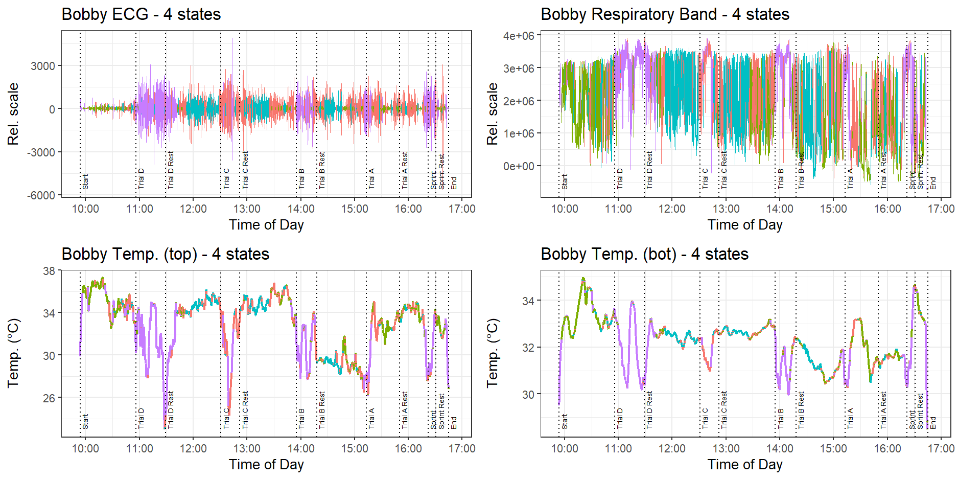
Figure 12 shows the effect of adding a fourth state. While the model clearly identifies when the dog is exercising, clustering these times in a purple state, it is not able to isolate the sprint as a higher-intensity activity compared to the lower-intensity trot exercises.
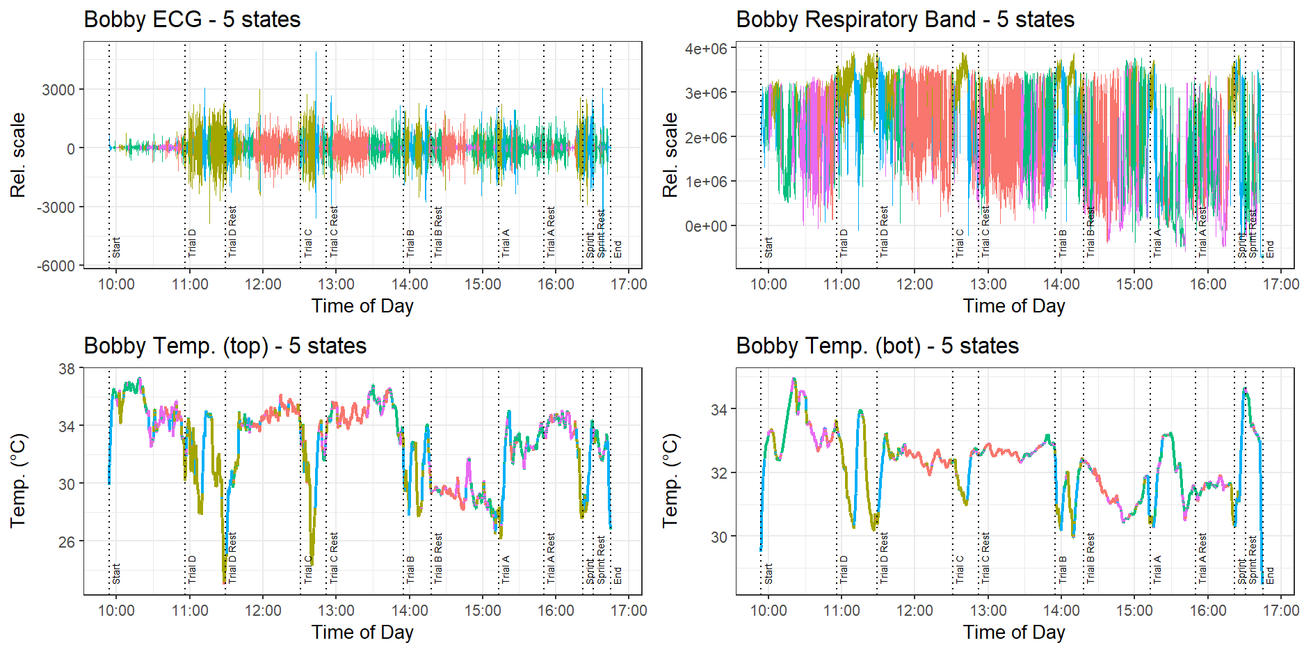
Moreover, the addition of a fifth state, as shown in Figure 13, does not improve matters - the HMM keeps breaking up the resting periods.
Discussion
Pill Data Discussion
The four and five-state HMMs fitted to the pill data were able to cluster the sprint exercise separately from the low-intensity trot exercises. However, the data from the pill showed sharp dips when the dog drank water, indicating that there are significant trade-offs with using the pill for analysing stress levels. In particular, the times when the dog wants to drink the most would be when it is performing high-intensity exercises, and that is exactly when we want the best data to make stress predictions, something the pill can’t guarantee if it’s affected by the dog drinking water.
However, if the dog is working independently of their handler, being able to detect when the dog is drinking water is still useful, not only because it is information that the handler would not be able to obtain otherwise, but also because the act of the dog drinking can itself hint to underlying heat stress and discomfort.
Harness Data Discussion
The harness data was substantially noisier than the pill data. As the dog moved, we could also observe the harness generating unintelligible data due to the sensors in the harness losing contact with the dog’s body. The poor quality of this data likely also led to our HMMs’ inability to cluster the higher-intensity sprint separately from the lower-intensity trot exercises, even with five hidden states. We believe that these disconnections and noise are caused by a poor harness fit, and unless this is addressed, would present major difficulties in a real-world deployment where a dog may be working independently and their handler may not be present to adjust their harness if it shifts out of place.
Future Directions
From our analysis, we have identified several directions for research and development.
- Improve Harness Fit: The data collected by the harness was not affected by the dog drinking water. Therefore, if we can develop a new harness that fits more comfortably and provides better contact between the sensors and the dog’s body, we may be able to collect higher-quality data that allows a multivariate HMM to separate the sprint state from the low-intensity trot exercises. Possibilities include investigating harnesses from different vendors or developing a bespoke harness that better integrates the required electronics.
- Adaptive Calibration Algorithms: Since it is unrealistic to expect perfect sensor contact, it would be useful to investigate methods of correcting for sensor drift over time, possibly including machine learning techniques (Tan et al. 2010).
- On the Fly Decoding: While we performed our analysis on the full dataset, there are alternative algorithms that successively classify data points as they are streamed in “on the fly”. It would be useful to investigate the practicality of these algorithms for real-time detection of heat stress.
Conclusion
In this work, we fitted univariate HMMs to internal body temperature data and multivariate HMMs to ECG, respiratory excursion and external temperature data collected by working dogs as they performed some exercises of varying intensity throughout the day. We determined that HMMs fitted to the dogs’ internal body temperature were able to cluster the sprint activity as a higher intensity state compared to the low-intensity trot exercises. However, the temperature-sensing pill used to collect this data recorded large dips in temperature when the dog drank water.
We also determined that the data collected by the harness was too noisy for the multivariate HMMs to isolate the sprint activity as separate from the low-intensity trot exercises. Some avenues for future research to improve the data collected by the harness include exploring methods of improving comfort and adaptive calibration algorithms. We also believe investigating on-the-fly decoding algorithms would also be useful in validating the real-world practicality of our approach.
Codes
The Expectation Maximisation Algorithm
Our implementation for fitting univariate HMMs was adapted from Visser & Speekenbrink (2022). The code is provided below.
# (Scaled) Forward Backward Algorithm implementation
fb <- function(tpm, densities, prior.probs, data)
{
  # Initialise the variables
  nt = length(data); nstates = nrow(tpm); A = tpm; B = densities
  beta = alpha = matrix(ncol = nstates, nrow = nt)
  ct = vector(length=nt)

  alpha[1, ] = prior.probs * B[1, ] # Calculate the forward probabilities

  ct[1] = 1/sum(alpha[1,])   # Compute the scaling variables

  alpha[1,] = ct[1] * alpha[1,] # Compute the scaled forward probabilities

  for (t in 1:(nt - 1)){
    # Use recursive structure of forward probabilities to calculate for each t
    alpha[t+1,] = (t(A) %*% alpha[t, ]) * B[t + 1, ]
    # Compute the scaling variables
    ct[t+1] = 1/sum(alpha[t+1,])
    # Compute the scaled forward probabilities
    alpha[t+1,] = ct[t+1] * alpha[t+1,] }
  # Compute the last scaled backwards variable
  beta[nt,] = ct[nt]

  for(t in (nt-1):1){
    # Use recursive structure of scaled backwards probabilities to calculate for each t
    for (i in 1:nstates)
    beta[t,] = (A%*%(B[t+1,]*beta[t+1,]))*ct[t] }

  # Compute the smoothing and filtering probabilities
  gamma = matrix(ncol = nstates, nrow = nt)
  xi = array(dim = c(nt-1, nstates, nstates))

  for (t in 1:nt){
    gamma[t,] = alpha[t, ] * beta[t, ] / ct[t] }

  for (t in 1:(nt-1)){
    for ( i in 1:nstates){
      for ( j in 1:nstates)
        xi[t, i, j] = alpha[t,i] * A[i,j] * B[ t+1, j] * beta[t+1, j]}}

  # Also calculate the log likelihood.
  loglikelis = -1*sum(log(ct))
  return(list(gamma = gamma, xi = xi, ct = ct, loglikelis = loglikelis ))
}

# Perform maximisation step for Gaussian components
# Using the filtering and smoothing probabilities
emMax <- function( gamma, xi , data ){

  # Initialise our variables
  nt = length(data)
  nstates = ncol(gamma)

  # Maximise with respect to transition probabilities matrix
  tpm = matrix(nrow = nstates, ncol = nstates)
  f = matrix( nrow = nstates, ncol = nstates )

  for (j in 1:nstates){
    for (k in 1:nstates){
      f[j,k] = sum(xi[,j,k]) }}

  for (j in 1:nstates){
    for (k in 1:nstates){
      tpm[j,k] = f[j,k]/ sum(f[j,]) }}

  # Maximise with respect to our state-dependent parameters
  sigmas = mus = vector(length = nstates)

  for(j in 1:nstates){
    mus[j] = sum(gamma[,j]*data)/sum(gamma[,j])
    sigmas[j] =  sqrt(sum(gamma[,j]*(data  - mus[j])^2 )/sum(gamma[,j]))
  }

  densities = matrix(nrow = nt , ncol = nstates)

  for(i in 1:nstates){
    densities[,i] = dnorm(data, mean = mus[i], sd = sigmas[i])
  }

  # Maximise with respect to our prior probabilities
  prior.probs = gamma[1,]

  return(list(tpm = tpm, densities = densities,
              prior.probs = prior.probs , mus = mus, sigmas = sigmas ))
}

# Perform the expectation maximisation step itself.
em <- function(data, nstates, MAXITER = 100){

  # Initialise starting values for EM
  nt = length(data)
  tpm = matrix(1/nstates, nrow = nstates, ncol = nstates)
  densities = matrix(nrow = nt , ncol = nstates)

  # Set up some initial values for our numerical solver
  for(i in 1:nstates){
    densities[,i] = dnorm(data, mean = mean(data), sd = sd(data))
  }

  v = runif(nstates)
  prior.probs = v/sum(v)

  # Define our convergence criteria.
  EPS = 1e-10
  ll = 100
  its = 0

  # Calculate our smoothing and filtering probabilities using forward backwards
  s = fb(tpm = tpm, densities = densities,
         prior.probs = prior.probs, data = data)
  t = emMax(s$gamma, s$xi, data)

  # Hill climb with the maximisation step and forwards-backwards algorithm until convergence
  for (ITER in 1:MAXITER){
    its = ITER
    s = fb(t$tpm, t$densities,
             t$prior.probs, data = data)
    t = emMax(s$gamma, s$xi, data = data)
    ll_new = s$loglikelis

    if( abs(ll_new - ll) < EPS){
      s <- paste("Converged in", ITER, "iterations.")
      message(s)
      break
    } else {
      ll = ll_new }
  }

  if(its == MAXITER){
    message("Model failed to converge in given iterations")
  }

  k = nstates*(nstates+2) - 1

  aic = 2*k - 2*ll
  bic = k*log(nt) - 2*ll
  metrics = c(aic,  bic, ll, df = k)

  names(metrics) = c("aic", "bic", "loglikelis", "df")
  return(list( tpm = t$tpm, prior.probs = t$prior.probs,
               mus = t$mus, sigmas = t$sigmas, densities = t$densities,
               metrics = metrics))
  }

# Implement the Viterbi algorithm described in Section 2.4
viterbi <- function(tpm, densities, prior.probs, data)
{
  A = tpm
  B = densities
  nstates = nrow(tpm)
  nt = nrow(densities)

  # Initialise variables
  delta = psi = matrix(nrow = nt, ncol = nstates)

  # Set initial condition
  delta[1,] = log(prior.probs * B[1,])
  psi[1,] = 0

  # Loop:
  for( t in 2:nt ){
    for( i in 1:nstates){
      delta[t,i] = log(B[t,i]) + max( delta[t-1,] + log(A[,i]))
      psi[t,i] = which.max( delta[t-1,] + log(A[,i]) )
    }}

  st_global = vector(length = nt)
  st_global[nt] = which.max(delta[nt,])

  # Backwards pass
  for (t in (nt-1):1){
    st_global[t] = psi[t+1, st_global[t+1]]
  }
  return(st_global)
}
References
Becker, M., (2011) Why do dogs pant? Available at:
https://www.vetstreet.com/dr-marty-becker/dog-behavior-decoded-why-do-dogs-pant
(Accessed 10/12/23)
Chatterjee, S., Thakur, R. S., Yadav, R. M., Gupta, L., Raghuvanshi, D. K., ‘Review of noise removal techniques in ECG signals,’ IET Signal Processing, 14(9), 569-590.
DeRuiter, S. L., Langrock, R., Skirbutas, T., Goldbogen, J.A., Calambokidis, J. Friedlaender, A. S., Southall, B. L., (2017) ‘A Multivariate Mixed Hidden Markov Model for Blue Whale Behaviour and Responses to Sound Exposure,’ The Annals of Applied Statistics, 11(1), 362-392.
Fletcher, R. (1987). Practical methods of Optimisation, 2nd Ed. Wiley: NY
Gordon, L. (2017). Hyperthermia and Heatstroke in the Working Canine (pp. 1–15). USAR Veterinary Group.
Jin, Y., Qin, C., Liu, J., Li, Z., Liu, C., ‘A novel deep wavelet convolutional neural network for actual ECG signal denoising’ Biomedical Signal Processing and Control, 87(A), 105480 doi.org/10.1016/j.bspc.2023.105480
Ligges, U., Short, T., Kienzle, P., Schnackenberg, S., Billinghurst, D., Borchers, H-W., Carezia, A., Dupuis P., Eaton, J. W., Farhi, E., Habel, K., Hornik, K., Krey, S., Lash, B., Leisch, F., Mersmann, O., Neis, P., Ruohio, J., Smith III, J. O., Stewart, D., Weingessel, A. (2023) signal: Signal Processing, R package, current version available from CRAN
Mastrantonio, G., Grazian, C., Mancinelli, S., & Bibbona, E. (2019). ‘New formulation of the logistic-Gaussian process to analyze trajectory tracking data,’ The Annals of Applied Statistics, 13(4), 2483-2508.
O’Brien, C., Tharion, W. J., Karis, A. J., & Sullivan, H. M. (2020). ‘Predicting military working dog core temperature during exertional heat strain: Validation of a Canine Thermal Model,’ Journal of Thermal Biology, 90, 102603. doi:10.1016/j.jtherbio.2020.102603
Pohle, J., Langrock, R., van Beest, F. M., & Schmidt N. M., (2017) Selecting the Number of States in Hidden Markov Models: Pragmatic Solutions Illustrated Using Animal Movement. Journal of Agricultural, Biological, and Environmental Statistics, 22(3) 270-293.
R Core Team (2021). R: A language and environment for statistical computing. R Foundation for Statistical Computing, Vienna, Austria. https://www.R-project.org/.
Roebuck, P., (2014) rwt: Rice Wavelet Toolbox Wrapper., R package, archived: accessible from https://cran-archive.r-project.org/web/checks/2023/2023-01-09_check_results_rwt.html
Starling M., Jayarathna, T., Grazian, C., Contractor, S., Flower, B., Lomax, S., Breen, P., Sisson, S., Jay, O., Leong, P., Clark, C., McGreevy, P., Broderik, C., (2022) ‘Optimising Australian Defence Force military working dog performance through next generation monitoring systems,’ Defence Innovation Network
Tan. R., Xing. G., Liu, X., Yao J., & Yuan, Z., (2010) ‘Adaptive Calibration for Fusion-based Wireless Sensor Networks,. Proceedings IEEE INFOCOM, pp. 1-9, doi:10.1109/INFCOM.2010.5462036.
(Capt.) Thomas, K. (2022) ‘Military police welcome new hounds and handlers,’ Australian Government - Department of Defence. Available at:
https://www.defence.gov.au/news-events/news/2022-10-21/military-police-welcome-new-hounds-and-handlers
(Accessed 20/02/24)
Visser I. & Speekenbrink M. (2022) Mixture and Hidden Markov Models with R. Springer: Switzerland
Visser I, Speekenbrink M (2010) depmixS4: An R-package for hidden Markov models. J Stat Softw 36(7):1–21. http://www.jstatsoft.org/v36/i07/, R package, current version available from CRAN
Zucchini W., MacDonald I. L., Langrock, R., (2016) Hidden Markov Models for Time Series. CRC Press: FL