Hidden Markov Models for Analysing Stress Levels in Working Dogs
\(\newcommand{\Bf}[1]{\mathbf{#1}}\) \(\newcommand{\Bs}[1]{\boldsymbol{#1}}\)
Supervised by A/Prof Clara Grazian ~ March 2024
This is a short summary and introduction to the work. For the full project, see here.
Table of Contents
Background
As our best friends, we rely on dogs for some very important and strenuous tasks. For example, we have trained dogs to herd sheep and cattle, perform search and rescue operations, and even help in the military.
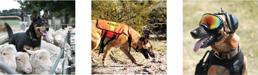
Especially in Australia however, where the climate is very hot, these tasks may put the dogs at a high risk of heat stress. This is a challenge for dog handlers, because working dogs, like Kelpies, are bred to be highly resilient and hardworking, so they do not exhibit warning signs until it becomes dangerous. Moreover, different dogs, even of the same breed, and under the same environmental conditions, may have very different responses. Of course, dogs may be working out of the sight of their handlers as well.
These factors make it very hard for handlers to judge a dog’s wellbeing by qualitative means. For this reason, it is useful to be able to detect the signs of overtemperature stress using a quantitative approach.
Experimental Setup
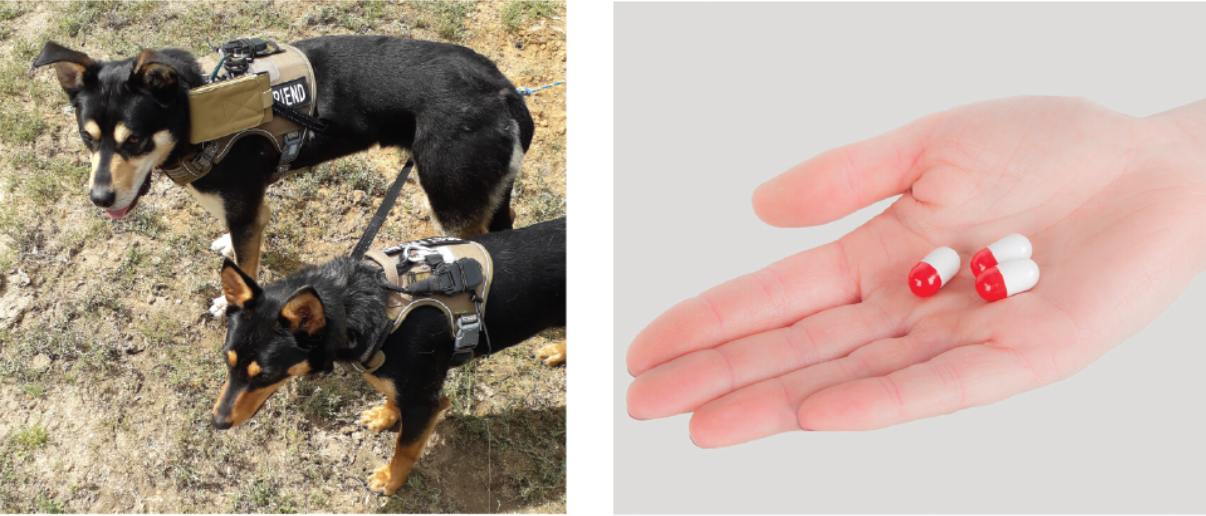
In order to test any machine learning algorithm however, we need some data. To collect it, we fitted six kelpies with a harness recording their ECG patterns, respiratory excursions, acceleration and temperature at each dog’s back and belly. Each dog also ingested a pill that measured their internal body temperature.
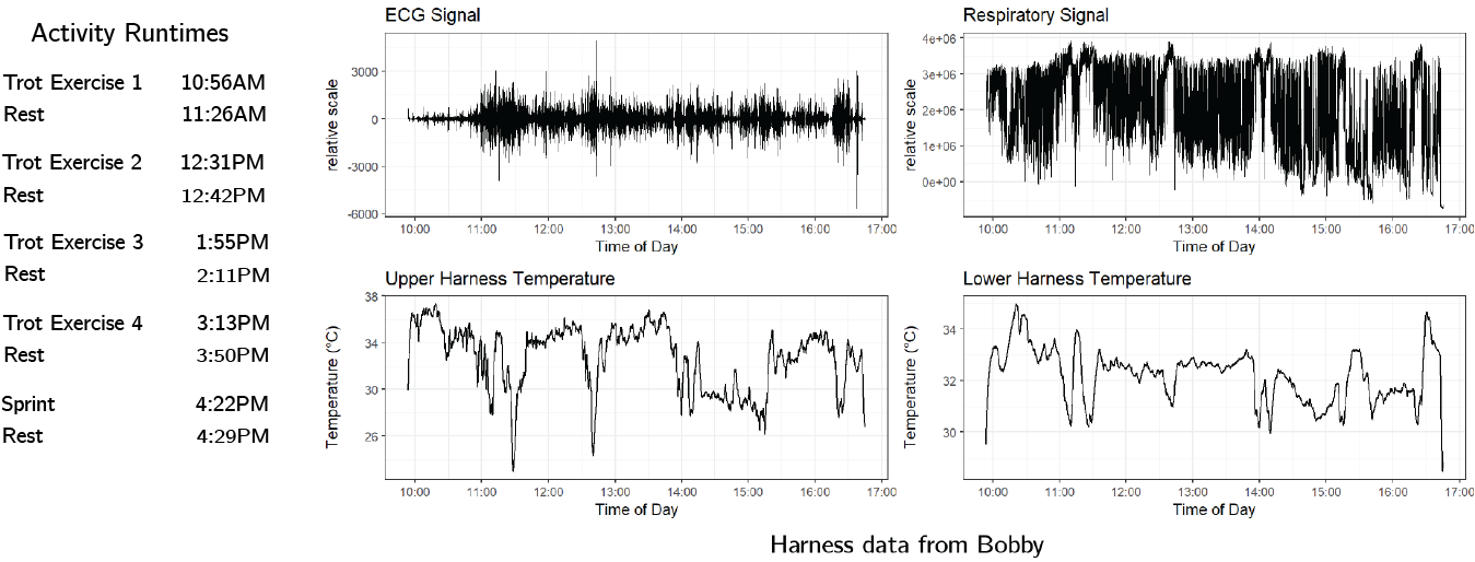
The dogs where then given a set of activities to perform throughout the day. The sprint exercise is the most intense activity, and ideally we should be able to detect it within the data as its own “high intensity activity” state. The graphs below show the data collected from Bobby’s harness. It is clear that the recorded signals are very noisy.
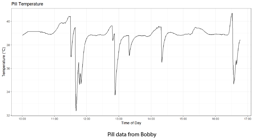
We also have the data collected from Bobby’s temperature sensing pill. This data has a lower frequency, and appears smoother.
From this data, we want to be able to infer the behavioural stress of the dog, and in particular, whether the dog is in a high activity state and hence at a heightened risk of heat stress.
Hidden Markov Models
First, we introduce some terminology. Represent the current behavioural state of the dog at time $t$ out of $N$ possible states by the random variable $S_t\in \{1,\dotsb, N\}$. For example, we might say that our dog has two behavioural states $\{1,2\}$ where state $1$ is “sleepy” and state $2$ is “excited”, and $S_t = 1$ would mean that at time $t$ the dog is sleepy.
Next, we say that the state sequence $S_{1:T} = (S_1,\dotsb,S_T)$ satisfies the Markov Property if
\[P(S_{t+1}\mid S_{1:(t)}) = P(S_{t+1} \mid S_{t})\,,\]that is, our prediction about the future behavioural state of the dog depends only on the present behavioural state, and not the sequence of events preceeding it.
We will associate with the state sequence $S_{1:T}$ with an initial probabilites vector
\[\boldsymbol{\theta}_{\text{init}} = \big [ P(S_1 = 1), P(S_1=2), \dots, P(S_1=N)\big ] \,.\]which encodes for the probabilities of the dog being in each behavioural state at the initial time.
We also need to define a transition probabilities matrix: a matrix $\boldsymbol{\theta}_{\text{trans}_{N\times N}}$ such that
\[\boldsymbol{\theta}_{\text{trans}_{i,j}} = P(S_t = i \mid S_{t-1}= j)\,.\]The transition probabilities matrix encodes for how the dog moves between different behavioural states. Considering the frequency of our data, we ideally want to see large diagonal entries in this matrix to indicate the presence of stable states.
Now, we can represent the observation at time $t$ by the random variable $X_t$, and associate with $X_{1:T}=(X_1,\dots,X_T)$ some distribution parameters $\boldsymbol{\theta}_{\text{obs}}$. For example, we might say $X_1\sim\mathrm{Normal}(0,1)$ and $X_2\sim \mathrm{Normal}(2,3)$, so these pairs of mean and variances would be stored in $\boldsymbol{\theta}_{\text{obs}}$. Note that $X_t$ could be a scalar or a random vector as well.
At this stage, we can finally define a Hidden Markov Model.
Definition (Hidden Markov Model)
A Hidden Markov Model (HMM) is defined by two sequences
- A state sequence \( S_{1:T} \) satisfying the Markov property.
- A response sequence \( X_{1:T} \) satisfying the conditional dependence \[ f(X_t \mid S_{1:t} , X_{1:t-1} ) = f(X_t \mid S_t) \,. \]
As an example, suppose again we have two states $\{1,2\}$ representing sleepy and excited respectively. We might expect to see the following structure:
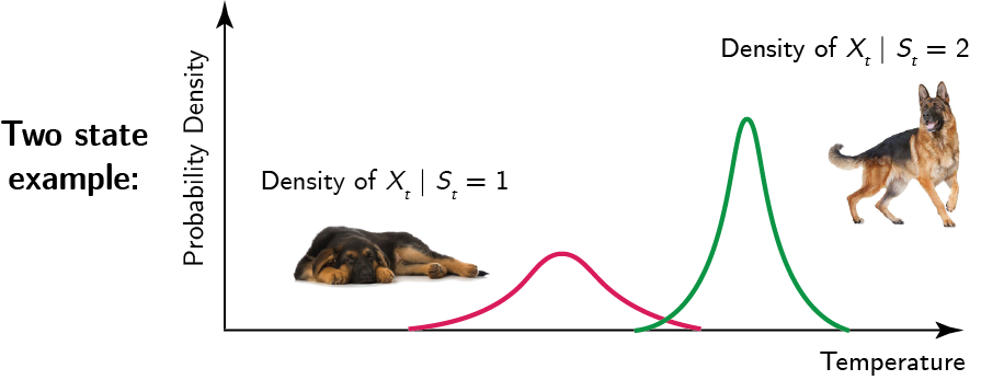
The probability density of the dog’s body temperature is probably lower when sleeping in state $1$ compared to when the dog is excited and playing around in state $2$. For this reason, the probability density of the body temperature $X_t$ takes on a different shape and location depending on whether the dog is sleeping or excited.
The challenge of course is that we do not always know the underlying behavioural state of the dog – this information is “hidden” from us. We would therefore need to infer the underlying state using the observed sensor data.
Performing Inference with Hidden Markov Models
Given a vector of observations $x_{1:T}$, and assuming there are $N$ possible states, we need to first estimate the parameters $\Bs{\theta}_{\text{init}}$, $\Bs{\theta}_{\text{tran}}$ and $\Bs{\theta}_{\text{obs}}$, collectively $\Bs{\theta}$ before we can perform inference on the hidden behavioural state sequence.
We do this by maximising the likelihood function, given by
\[L(\Bs{\theta}) = \sum_{i=1}^Nf(x_{1:T} ,S_T=i\mid \Bs{\theta}) \,.\]There are two main ways of doing this in the literature. One can simply perform direct maximisation using a numerical optimiser. There is also the Expectation Maximisation algorithm which takes advantage of the conditional structure of the hidden Markov model.
Suppose that we have implemented one of these methods, and have estimated the parameters $\Bs \theta$ of our model. Then, we can decode the most probable hidden state sequence using the Viterbi Algorithm.
The Viterbi Algorithm relies on two components. We first calculate the Forward Pass variable, which contains, given the observed data up to the present time $t$, the likelihood of the most likely sequence that ends at state $S_t = j$ at time $t$.
\[\alpha_{t}(j) := \underset{s_{1:(t-1)}}{\mathrm{max}} f(S_{1:(t-1)} = s_{1:(t-1)}, S_t = j, x_{1:t}) \,.\]To compute the forward pass variable, we can exploit the following recursion
\[\alpha_{t+1}(i) = f(x_{t+1} \mid S_{t+1} =i) \cdot \underset{j} {\mathrm{max}} \ P(S_{t+1} = i \mid S_t =j)\alpha_{t}(j) \,.\]Next, we compute the reverse pass variable, which contains at each time $t$, for each possible state $i$, the most likely state at time $t-1$ that preceeded it.
\[\beta_{t}(i) := \underset{j}{\mathrm{argmax}} \ \alpha_{t-1}(j) P(S_t = i\mid S_{t-1}=j)\]Computing the foward pass and reverse pass variables allows us to decode the hidden state sequence via the Viterbi algorithm.
The idea, described in more detail in the report, is to
- Keep track of the most likely possible state sequences that end in state $i$ for each $i=1,\dots, N$ at each time $t=1,\dots, T$, while also keeping track of the reverse pass variables.
- Assign the final state $S_T$ to be the state that the hidden Markov model is most likely to reach, that is, $\tilde{s}_T \gets \underset{i}{\mathrm{argmax}}(\alpha_{T}(i))$.
- Use the information stored in the reverse pass variables to estimate the most likely state at time $T-1, T-2,\dots, 1$ until the entire state sequence has been decoded, so $\tilde{s}_t \gets \beta_{t+1}(\tilde{s}_{t+1})$.
Now we can estimate the hidden state sequence of a hidden Markov model! 😊
The full report details our findings when we applied these algorithms to the dogs’ harness and pill sensors.