Bayesian Model Selection for Logistic Regression via Approximate Bayesian Inference
\(\newcommand{\Bf}[1]{\mathbf{#1}}\) \(\newcommand{\Bs}[1]{\boldsymbol{#1}}\) \(\newcommand{\KL}[0]{\mathrm{KL}}\) \(\newcommand{\apxpropto}{\underset{\sim}{\propto}}\)
Supervised by A/Prof John Ormerod ~ Dec 2023
For a summary of the project, see here.
For the complementary R package, see here.
Abstract
We apply variational Bayes and reverse collapsed variational Bayes methodologies to perform simultaneous model selection and coefficient estimation in the logistic regression context. We then explore the effect of the model’s hyperparameters on properties like model sparsity and compare our RCVB model’s cross-validation performance to some alternative reduced models derived from stepwise AIC on low-dimensional data. We also compare against some random forest and $k$-NN models on high-dimensional data.
Table of Contents
Introduction
Logistic regression, popularised by Berkson (1951), is a widely used linear method for modelling the relationship between numerical predictors $\Bf X$ and a binary response $\Bf y$. It is used in a wide range of applications, for example predicting whether a patient will develop a particular disease given observations of their body and health, and predicting whether a component will fail given certain working conditions.
Suppose we have $n$ independent observations of $p$ predictors with $n$ corresponding responses. Encoding this information as
\[\Bf X = \begin{bmatrix} 1 & \verb|predictor_1|_1 & \cdots &\verb|predictor_p|_1 \\ \vdots & \vdots & \ddots & \vdots \\ 1 & \verb|predictor_1|_n& \cdots & \verb|predictor_p|_n \\ \end{bmatrix} \text{ and } \Bf y =\begin{bmatrix} y_1 \\ \vdots \\ y_n \,,\\ \end{bmatrix}\]where $y_i \in {0,1}$ represents the binary response, we fit coefficients $\Bs \beta = (\beta_0,\dotsb, \beta_p)$ so the logistic curve \begin{equation} \mathrm{expit}(\Bf X \Bs \beta) := \frac{e^{\Bf X \Bs \beta}}{ 1 + e^{ \Bf X \Bs \beta}} \,. \end{equation} models the probability that the components of $\Bf y$ are equal to $1$. In a classification framework, for an observation $\Bf x’$, we predict the response $y’= 1$ if $\mathrm{expit}(\Bf x’ \Bs \beta) > 0.5$ and $0$ if $\mathrm{expit}(\Bf x’ \Bs \beta) < 0.5$. If $\mathrm{expit}(\Bf x’ \Bs \beta) =0.5$, a possible tie-break rule could be to assume it is the majority response in $\Bf y$. (Tarr, 2023)
The standard way of computing the coefficients of $\Bs \beta$ involves maximising a likelihood function numerically (Hosmer and Lemeshow, 1989). However, this method runs into stability issues with high dimensional data, that is, when $p>n$.
An alternative framework for parameter estimation comes courtesy of Bayesian inference. If we assume the prior distribution of a parameter $\Bs \theta$, and observe data $\Bf x$, we can derive a posterior, or updated, distribution of $\Bs \theta \mid \Bf x$ using Baye’s Rule:
\begin{equation} p(\Bs \theta \mid \Bf x) =\frac{p( \Bf x \mid \Bs \theta ) p(\Bs \theta)}{ \int_{\Omega} p(\Bf x \mid \Bs \theta ) p(\Bs \theta) d\Bs \theta }\,, \end{equation}
where $\Bs \theta \in \Omega$ is the parameter space. One possible prediction for $\Bs \theta$ is the mode of $p(\Bs \theta \mid \Bf x)$, with a prediction made this way called the Maximum a Posteriori (MAP) estimate. However, the integral in the denominator is often intractable and therefore requires approximation. There are two main methodologies in the literature.
The historically more dominant method is Markov Chain Monte Carlo (MCMC) sampling. (Hastings, 1970; Gelfand and Smith, 1990). MCMC methods involve constructing a Markov chain to sample from the posterior distribution. After a sufficient number of steps, the chain reaches an equilibrium where the probabilities of being in each state are constant, allowing us to obtain samples representative of our desired posterior. While MCMC methods are asymptotically exact, the number of samples required to obtain sufficient accuracy may be computationally impractical for large datasets.
As a result, we will focus on the main alternative: Variational Bayesian (VB) inference. Ormerod and Wand (2010) provides an overview of the statistical basis of VB methods and several motivating examples. Instead of sampling, the idea is to reduce the intractable integral into an optimisation problem. For a density $q$, we can define the Kullback-Leibler ($\KL$) divergence to the posterior by the integral
\begin{equation} \label{eq:KL} \KL(q(\Bs \theta),p(\Bs \theta \mid \Bf x)) = \int q(\Bs \theta) \log\left(\frac{q(\Bs \theta)}{p(\Bs \theta \mid \Bf x)}\right) d\Bs \theta \,. \end{equation}
The goal is to compute the optimal density $q^*(\Bs \theta)$ that minimises $\KL(q(\Bs \theta),p(\Bs \theta \mid \Bf x))$ and then use $q^*(\Bs \theta)$ as an approximation of the posterior density. In practice, VB methods are significantly faster than MCMC sampling. However, its approximations are not guaranteed to be exact.
Recently, Yu, Ormerod and Stewart (2020) introduced an extension to VB, coined Reverse Collapsed Variational Bayes (RCVB), where the idea is to perform VB fits to a subset of the parameters, and then collapse the remaining parameters by marginalising over the joint density.
Another important consideration when building predictive models is the task of model selection. In datasets with many predictors, it is often the case that only a subset of them will carry meaningful information about the response. The goal of model selection is to find these predictors. In practice, logistic models regressing on this reduced subset of predictors are less prone to overfitting and are easier to understand.
The classical approach to model selection involves calculating the Wald test statistic for each predictor, and using the $\chi^2$ distribution of the Wald statistic to assign each predictor a $p$-value. Alternatives include stepwise model selection algorithms, which compare different models to find the best fit by iteratively adding or removing predictors based on some information or complexity criterion like AIC.
To adapt model selection to the Bayesian context, Ormerod, You and Müller (2017) instead considered the logistic model
\begin{equation}
\mathrm{expit}(\Bf X \mathrm{diag}(\Bf w) \Bs \beta) := \frac{e^{\Bf X \mathrm{diag}(\Bf w) \Bs \beta}}{ 1 + e^{ \Bf X \mathrm{diag}(\Bf w) \Bs \beta}} \,,
\end{equation}
where $\Bf w = (w_0,\dotsb, w_p)$ is a “binary mask” with coefficients $w_i\in {0,1}$. When $w_i = 0$, the effect of the $i$-th predictor is dropped from the regression, and when $w_i = 1$, then the effect is included. We can use VB and RCVB methods to estimate the coefficients of $\Bf w$, the model selection vector.
Aims
Our main aim for this report is to apply VB and RCVB methods to the parameter estimation problem of logistic regression. Given observational data $\Bf X$ and a binary response vector $\Bf y$, we aim to find approximate posterior densities for the regression coefficients $\Bs \beta = (\beta_0,\dotsb, \beta_p)$ where the coefficients have prior density $\beta_j \sim \mathrm{Normal}(0,\sigma^2)$ and model selection matrix $\Gamma = \mathrm{diag}(\gamma_0,\dotsb, \gamma_p)$ where the diagonal entries have prior density $\gamma_j \sim \mathrm{Bernoulli}(\rho)$. To perform classification, we will use the MAP estimates.
We also aim to apply repeated cross-validation to tune the hyperparameters $\sigma$ and $\rho$, and to compare the out-of-sample performance of our tuned model with alternative approaches on both low-dimensional and high-dimensional datasets.
Methods
Variational Bayes Algorithm
To minimise the $\KL$ divergence from the posterior of $\Bs \theta$ as defined by \ref{eq:KL} in a sensible way, we need to impose restrictions on the allowed forms of the $q(\Bs \theta)$ density. Following Ormerod and Wand (2010), we impose a mean field restriction, which states the density $q(\Bs \theta)$ must factor into
\begin{equation} \label{eq:mfa} q(\Bs \theta) = \prod_{i=1}^Mq_i(\Bs \theta_i) \,, \end{equation}
for some partition $(\Bs \theta_1,\dotsb,\Bs \theta_M)$ of $\Bs \theta$. If we do so, then the individual factors have optimal density
\begin{equation} \label{eq:opt} q_i^*(\Bs \theta_i) \propto \exp\left[E_{-\Bs \theta_i}\log(p(\Bf x,\Bs \theta))\right] \,, \end{equation}
for $i=1,\dotsb,M$ where $E_{-\theta_i}$ is the expectation with respect to the density $\prod_{j\neq i}q_j(\Bs \theta_j)$. (Ormerod and Wand 2010)
We can now apply this theory to the logistic regression experiment described in the Aims. For each $i=1,\dotsb,n$, let $Y_i$ be a random variable with image points in ${0,1}$ corresponding to the coefficient $y_i$ in the response vector $\Bf y$. The probability that $Y_i =1$, given observation $\Bf x_i$ (the $i$-th row of data matrix $X$), regression coefficients $\Bs \beta$ and model selection matrix $\Gamma$ is
\begin{equation} \pi_i := P(Y_i = y_i\mid \Bf x_i, \Bs \beta, \Bs \Gamma) = \mathrm{expit}(\Bf x_i^T \Bs \Gamma \Bs\beta) \,. \end{equation}
For each $i$ then, we have $P(Y_i = y_i \mid \Bf{x}_i, \Bs \beta, \Bs \Gamma) = \pi_i^{y_i}(1-\pi_i)^{1-y_i}$. For $\Bf Y= (Y_i,\dotsb, Y_n)$, define the likelihood to be the product
\begin{equation} \label{eq:likelis} L(\Bs \beta) := P(\Bf Y= \Bf y \mid \Bf X,\Bs \beta, \Bs \Gamma) = \prod_{i=1}^{n}\pi_i^{y_i}(1-\pi_i)^{1-y_i} \,. \end{equation}
If we take the logarithm of both sides, we get
\[\begin{equation} \label{eq:loglikelis} \ell(\Bs \beta) := \log\left(\prod_{i=1}^{n}\pi_i^{y_i}(1-\pi_i)^{1-y_i}\right) = \Bf{y}^T \Bf{X} \Bs \Gamma \Bs \beta - \Bf{1}^T\log( \Bf{1} + \exp(\Bf{X} \Bs \Gamma \Bs{\beta})) \,. \end{equation}\]To apply Formula \ref{eq:opt}, we will use the partition $(\Bs \beta, \Bs \Gamma) = (\Bs \beta, \gamma_0,\dotsb, \gamma_p)$. The optimal $\beta$ density is therefore
\[\begin{aligned} q(\Bs \beta) &\propto \exp{[E_{-\Bs \beta} (\ell(\Bs \beta) + \log p(\Bs \beta) + \log p(\Bs \gamma) )]} \end{aligned}\]where substituting our prior densities, we obtain
\begin{equation} q(\Bs \beta) \propto \exp \Big[ \Bf y^T \Bf X \Bf W \Bs \beta - E_{\Bs \gamma} (\left(\Bf 1^T \log(\Bf 1 +\exp(\Bf X\Bs \Gamma \Bs \beta) \right) \ -\frac{1}{2\sigma^2}| \Bs \beta |^2 \Big] \,. \end{equation}
where $\log p(\Bs \gamma)$ was absorbed into the constant of proportionality. Here, we also define $w_j = q(\gamma_j = 1)$ and $\Bf W=\mathrm{diag}(w_0,\dotsb,w_p)$ to be the MAP estimate of the model selection coefficients. To approximate the expectation $E_{\Bs \gamma}\left[\Bf 1^T \log(\Bf 1 +\exp(\Bf X\Bs \Gamma \Bs \beta)) \right]$ we use the $\delta$-method. The idea is to use a Taylor expansion for the log density. In our case, a first-order approximation will suffice:
\[\begin{equation} \label{eq:delta1} E[f(x)] \approx E[f(\mu) + \nabla f(\mu) (x-\mu)] = f(\mu) \,. \end{equation}\]Applying Equation \ref{eq:delta1} here, we have the following approximation
\[E_{\Bs \gamma}\left[\Bf 1^T \log(\Bf 1 +\exp(\Bf X\Bs \Gamma \Bs \beta) \right] \approx \Bf 1^T \log(\Bf 1 +\exp(\Bf X\Bf W \Bs \beta)) \,.\]Hence we obtain
\[\begin{equation} \label{eq:beta_update_vb} q(\Bs \beta) \apxpropto \exp\Big[ \Bf y^T \Bf X \Bf W \Bs \beta - \Bf 1^T \log(\Bf 1 +\exp(\Bf X\Bf W \Bs \beta) ) -\frac{1}{2\sigma^2}\| \Bs \beta \|^2 \Big] \,. \end{equation}\]Using the Laplace approximation (MacKay, 2003), we can approximate the posterior density of $\Bs \beta$ by
\begin{equation} \Bs \beta \sim \mathrm{Normal}( \widetilde{\Bs \beta} , \widetilde{\Bs \Sigma}) \,, \end{equation}
where $\widetilde{\Bs \beta} = \mathrm{argmax}(f(\Bs \beta))$, $\widetilde{\Bs \Sigma} = [-\nabla^2f(\Bs \beta)]^{-1}_{\Bs \beta = \widetilde{\Bs \beta}}$ and
\begin{equation} \label{eq:f} f(\Bs \beta) = \Bf y^T \Bf X \Bf W \Bs \beta - \Bf 1^T \log(\Bf 1 +\exp(\Bf X\Bf W \Bs \beta)) -\frac{1}{2\sigma^2}| \Bs \beta |^2 \,. \end{equation}
In our implementation, we performed this maximisation using a Newton-Raphson scheme. Now, we consider the densities $q(\gamma_j)$ where $j=0,\dotsb,p$. We have
\begin{equation}
q(\gamma_j) \propto \exp E_{-\gamma_j}\left(\Bf y^T \Bf X \Bs \Gamma \Bs \beta - \Bf 1^T \log(\Bf 1+\exp(\Bf X \Bs \Gamma \Bs \beta)) + \gamma_j \log\left(\frac{\rho}{1-\rho}\right) \right) \,,
\end{equation}
where we define
\[E_{-\gamma_j}\left(\Bf y^T \Bf X \Bs \Gamma \Bs \beta \right) = E_{\beta, \gamma_{-j}}\left(\Bf y^T \Bf X \Bs \Gamma \Bs \beta \right) = (\Bf X^T \Bf y)_j \gamma_j \mu_j \,.\]By another application of the $\delta$-method, we obtain
\begin{equation}
E_{\Bs \beta, \gamma_{-j}}\left(1^T \log(1+ \exp(\Bf X \Bs \Gamma \Bs \beta)) \right)
\approx 1^T \log(1+\exp{[X_j \gamma_j \mu_j + X_{-j} W_{-j}\mu_{-j}]})\,,
\end{equation}
where $\mu_j$ is the expectation of $\beta_j$. Bringing it together, we have
If we define
we can rewrite
\[q(\gamma_j) = z_j \exp(\tau(\gamma_j))\]where $z_j$ is some normalising constant. Nevertheless, $q(\gamma_j =1)=z_j \exp(\tau(1))$ and $q(\gamma_j = 0)=z_j \exp(\tau(0))$ so we have
\[q(\gamma_j = 0) + q(\gamma_j = 1) = 1 \implies z_j = \frac{1}{\exp(\tau(0)) + \exp(\tau(1))}\,,\]and moreover,
\begin{equation} q(\gamma_j) = \frac{\exp(\tau(\gamma_j))}{\exp(\tau(0))+\exp(\tau(1))}\,. \end{equation}
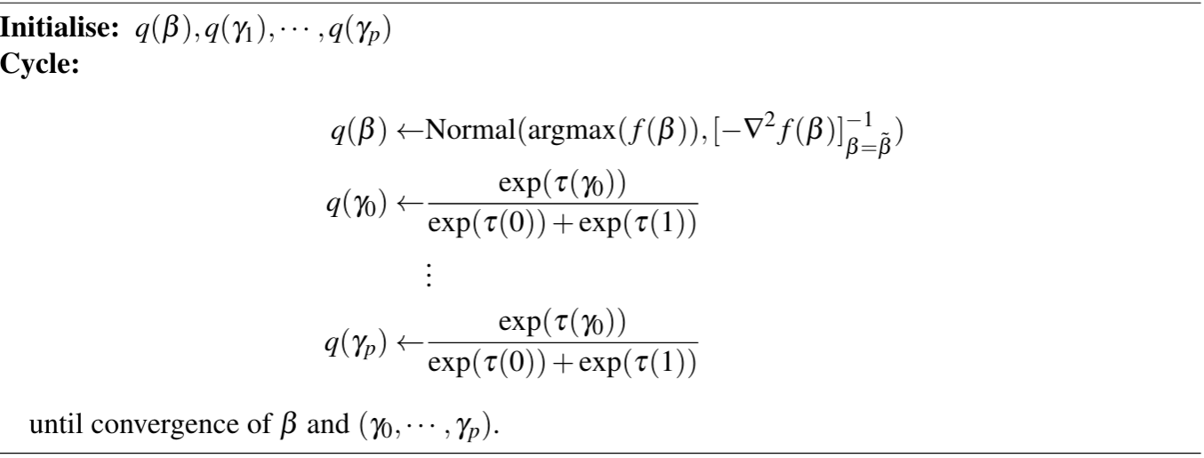
Using $f(\Bs \beta)$ defined as in Equation \ref{eq:f}, and $\tau(\gamma_j)$ defined as in Equation \ref{eq:tau_update_vb}, we can summarise our work by Algorithm 1.
Reverse Collapsed Variational Bayes (RCVB) Algorithm
An alternate way of approaching this problem is to apply RCVB to the model selection vector $(\gamma_0,\dotsb, \gamma_p)$: evaluating each coefficient at $\gamma_j=0$ and $\gamma_j=1$ and then combining the data by marginalizing over $\Bs \beta$. We will use the same partition and $\Bs \beta$ density as in the VB approach.
To compute $q(\gamma_j)$, again let $\Bf w$ be the vector $(w_0,\dotsb, w_p)$ where $w_i = E(\gamma_i)$. Denote
\begin{equation} \label{eq:wjk} \Bf w^{(j,k)} = (w_1, \dotsb, w_{j-1}, k, w_{j+1}, \dotsb, w_p) \end{equation}
where $k \in {0,1}$. We update our $\gamma_j$ using
We can approximate this integral, again using the Laplace approximation. Defining
where $\Bf Z^{(j,k)} = \Bf X\mathrm{diag}(\mathbf{w}^{(j,k)})$, we have
\begin{equation} \int \exp{g(\beta_k,k)} d\beta \approx \int \exp \left[ g(\hat{\beta}_k,k) + \frac12 (\beta-\hat{\beta})^T \nabla^2 g(\hat{\beta}_k,k) (\beta-\hat{\beta}) \right] d\beta \,, \end{equation}
where $\hat{\beta}_k = \mathrm{argmax}(g(\beta_k,k))$. By inspection, the covariance matrix of the $\Bs \beta$ normal approximation is given by $[-\Sigma^{-1}_k] = \nabla^2 g(\hat{\beta}_k,k) $. To evaluate this integral, we first factor out some constant terms
However, we have the following identity using the integral of the multivariate normal distribution
\begin{equation} \int_{\Omega} \exp{\left(-\frac12 (\theta- \mu)^T \Sigma^{-1}(\theta-\mu) \right)} d\theta = [\det{(2\pi \Sigma)]^{\frac12}} \,. \end{equation}
Upon matching terms, we have
so if we define $\kappa(k)$ to be the function such that $q(\gamma_j = k) = \alpha_j\exp(\kappa(k))$, then $\kappa$ satisfies, up to a constant $\alpha_j$,
\begin{equation} \label{eq:kappa} \kappa(k) = g(\hat{\beta}_k, k) - \frac12 \log{\det(\Sigma^{-1}_k)} + k\log(\rho/ 1-\rho) \,, \end{equation}
so we obtain
\begin{equation} \label{eq:cvb_gamma_update} q(\gamma_j =1) = w_j = \frac{|\Sigma_1|^{\frac12} \exp{\kappa{(1)}} }{|\Sigma_1|^{\frac12}\exp{\kappa{(1)}} + |\Sigma_0|^{\frac12}\exp{\kappa{(0)}}} \,, \end{equation}
where $\Sigma_k$ is the covariance matrix obtained from the $\Bs \beta$-update Laplace approximation with $\gamma_j = k$, for $k \in {0,1}$. Using $\kappa$ defined as in Equation \ref{eq:kappa}, and the same definitions for $q(\Bs\beta)$, we can again summarise our work in Algorithm 2.
Results
The Pima Indians diabetes dataset (pima) from Smith et al. (1988) is a collection of medical records from 768 Pima Indian women, which includes the health metrics shown in Table 1 and whether they tested positive or negative for diabetes.
| Predictor | Unit | Variable Name |
|---|---|---|
| No. of Pregnancies | n/a | pregnant |
| Glucose level | mg/dL | glucose |
| Blood Pressure | mmHg | pressure |
| Tricep Fold Thickness | mm | tricep |
| Insulin Level | muU/mL | insulin |
| BMI | n/a | bmi |
| Diabetes Pedigree | n/a | pedigree |
| Age | yrs | age |
Table 1. Predictors in pima dataset
Variational Bayes Approach Results
After running the VB algorithm on the Pima Indians dataset with untuned hyperparameters $(\sigma, \rho) = (10,0.1)$, we plotted the MAP estimates of the model selection coefficients through each iteration in Figure 1 (left) and the regression coefficients in Figure 1 (right).
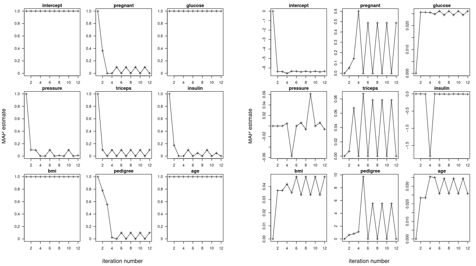
If the algorithm was operating correctly, then the MAP estimates $w_j$ of the approximate posterior $q(\gamma_j)$ should converge to either $0$ (excluding the predictor) or $1$ (including the predictor). Figure 1 (left) shows that while the coefficients for predictors deemed significant converged to $1$, the other predictors oscillated between $0$ and $\rho$ and did not converge. There is a similar oscillation in the $\mu_j$ values. We did not consider the VB model in our performance tests because of this failure to converge.
Reverse Collapsed Variational Bayes Approach Results
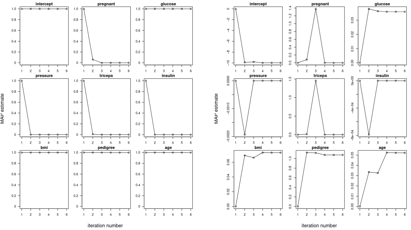
Running the RCVB algorithm on the Pima Indians dataset, with the same hyperparameters $(\sigma, \rho) = (10,0.1)$, we see significantly better convergence results. Figure 2 (left) shows the RCVB algorithm is capable of bringing the MAP estimates of the model selection coefficients corresponding to predictors deemed insignificant to $0$. Without the model selection coefficients oscillating, Figure 2 (right) indicates the regression coefficients are now able to converge.
Having verified that the RCVB model is working, we tuned the hyperparameters $(\sigma,\rho)$ by searching exhaustively in the space $(\sigma,\rho)\in{0.01,0.02\dotsb,0.99} \times { 1,2,\dotsb,20}$ for the pair of values that yielded the highest performance, which was measured by $10$-fold cross-validation with the metric
\[\mathrm{Error} = \frac{1}{10}\sum_{i=1}^{10}\left( \frac{1}{n_i} \sum_{j=1}^{n_i} 1_{\{h_{X_{\mathrm{train}}}(X_{\mathrm{test}, j}) = y_{\mathrm{test},j} \}} \right)\]where $h_{X_{\mathrm{train}}}$ is the classifier function representing our RCVB model fit on the training data and $1_{{h_{X_{\mathrm{train}}}(X_{\mathrm{test}, j}) = y_{\mathrm{test},j} } }$ is the indicator that the $j$-th prediction made on the test data is equal to the $j$-th observed response. For robustness, the cross-validation procedure was repeated $10$ times with the cross-validation error averaged to obtain the final value. The results are shown in the heatmap in Figure 3. Throughout this report, we will refer to the error computed this way as the “cross-validation error,” consistent with Tarr (2023).
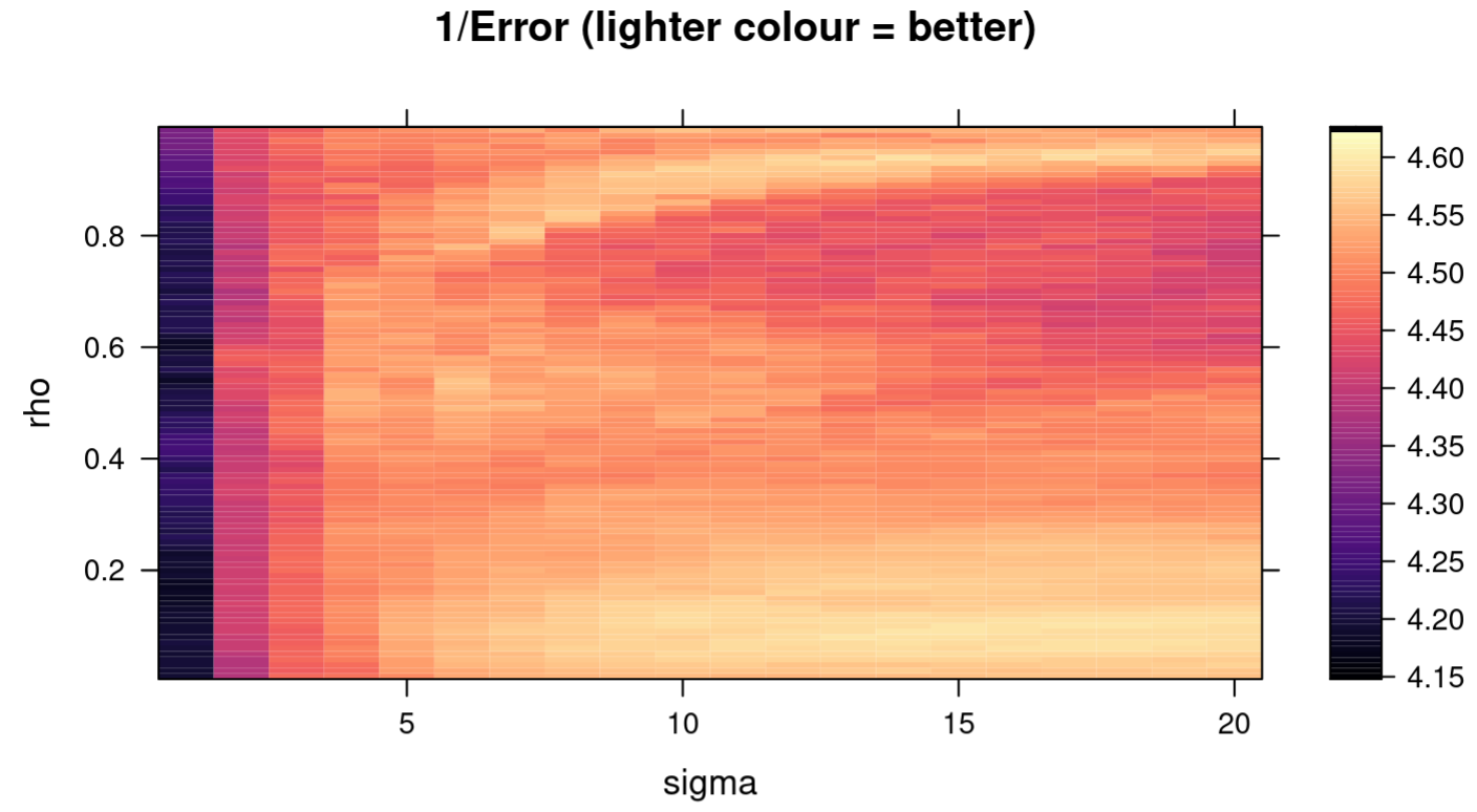
pima dataset.The pair $(\sigma, \rho) = (14,0.09)$ yielded the lowest averaged cross-validation error of $0.217$. While it is feasible to search through a finer grid, it is likely that any resolution beyond this point is noise and does not contribute meaningfully to the model. Using these hyperparameters, our final model selected for the predictors glucose, age, bmi and pedigree. It deemed the predictors pregnant, pressure, triceps and insulin not significant to predicting diabetes.
Results on Low Dimensional Data
For comparison, we devised some alternative models using the regsubsets function of the leaps package (Lumley and Miller, 2020), which exhaustively searches for the best set of predictors at each model size using stepwise methods. They are summarised along with our model in Table 2. A coefficient of $0$ indicates the variable is not significant.
| Predictor | Our Model (RCVB) | leaps Size 1 Model |
leaps Size 2 Model |
leaps Size 3 Model |
leaps Size 4 Model |
Full Model |
|---|---|---|---|---|---|---|
intercept |
-10.0296 | -6.0955 | -7.1640 | -9.6774 | -10.0920 | -10.040 |
pregnant |
0 | 0 | 0 | 0 | 0 | 0.0822 |
glucose |
0.0361 | 0.0424 | 0.0382 | 0.0363 | 0.0362 | 0.0383 |
pressure |
0 | 0 | 0 | 0 | 0 | -0.0014 |
triceps |
0 | 0 | 0 | 0 | 0 | 0.0122 |
insulin |
0 | 0 | 0 | 0 | 0 | 0.0008 |
mass |
0.0736 | 0 | 0 | 0.0779 | 0.0745 | 0.0705 |
pedigree |
1.0821 | 0 | 0 | 0 | 1.0871 | 1.1410 |
age |
0.0523 | 0 | 0.0506 | 0.0541 | 0.0530 | 0.0395 |
Table 2. Regression Coefficients for Selected Variables with pima dataset
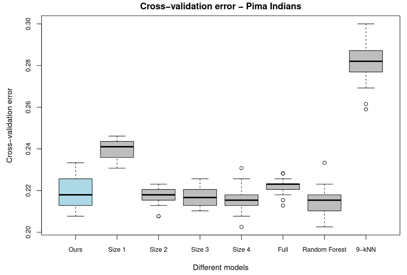
The cross-validation errors are plotted in Figure 4. We also compared our logistic model to some non-linear classifiers including a random forest with $500$ trees and a $k=5$-nearest neighbours model.
Note that we chose $k=5$ as it was the value recommended by the train function of the caret package (Kuhm, 2008) on the basis of repeated cross-validation performance.
pima datasetResults on High Dimensional Data
Our algorithm is flexible enough to be used on high-dimensional data, where the classical glm function will have trouble converging. However, $k$-nearest neighbours and random forests will still give sensible predictions.
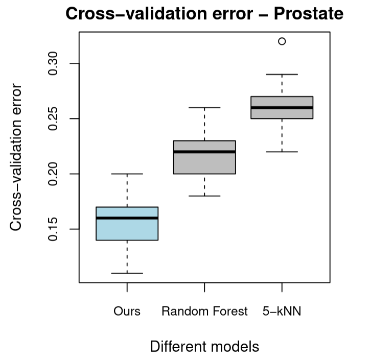
To test our model against these, we considered the Prostate Tumor Gene Expression (prostate) dataset used in Chung and Keles (2010). The original dataset consists of 52 prostate tumor and 50 normal tissue samples with $6033$ log-transformed and standardised gene expression levels taken from each sample as predictors. To reduce computational time, we used a random sample of $150$ gene expressions from the original dataset. Our RCVB algorithm with hyperparameters $(10,0.1)$ was able to converge in under $20$ iterations and determined $14$ of the gene expressions to be significant. Figure 5 provides a boxplot of cross-validation errors comparing our model with random forest and $k=9$-nearest neighbours, where $k=9$ was the value recommended by caret::train.
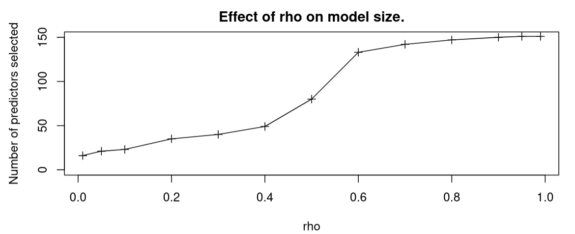
prostate datasetFigure 6 plots the number of variables selected for the reduced model against $\rho$. We see that as $\rho$ approaches $0$, the selected model approaches the null model, and as $\rho$ approaches $1$, the selected model approaches the full model.
Discussion
VB convergence analysis
The VB algorithm’s inability to converge was a setback for us. Analysis of the density updates showed that the oscillatory behaviour was intrinsic to the algorithm, and was not an issue of implementation.
To see this, consider the model selection coefficients plotted in Figure 1 (left). As expected, we see the algorithm trying to drive the coefficients of insignificant predictors to $0$ in the first few iterations. Let’s say that $w_j$ is one of the coefficients which becomes close to $0$. Figure 1 (right) shows the corresponding regression coefficient MAP estimate $\mu_j = E(\beta_j)$ will be sent to $0$ as well. That is because when searching for $\widetilde{\Bs \beta} = \mathrm{argmax}{f(\Bs \beta)}$ where $f$ is given in \ref{eq:f}, for $w_j\approx 0$, the $j$-th component of $\widetilde{\Bs \beta}$ does not contribute to the $\Bf y^T \Bf X \Bf W \Bs \beta - \Bf 1^T \log(\Bf 1 +\exp(\Bf X\Bf W \Bs \beta))$ term, and only to the negative $\frac{1}{2\sigma^2}| \Bs \beta |^2$ part.
To maximise $f(\Bs\beta)$ then, we require $\widetilde{\Bs \beta}_j = 0$. When the algorithm returns to compute the values of $\tau$, we obtain
\[\begin{aligned} \tau(0) &= -\Bf 1^T \log(1+\exp(X_{-j} W_{-j} \mu_{-j}))\\ \tau(1) &= -\Bf 1^T \log(1+\exp(X_{-j} W_{-j} \mu_{-j})) + \log{\left(\rho/1-\rho\right)} \,, \end{aligned}\]and substituting these expressions into \ref{eq:vb_gamma} we see that
\[\begin{equation} w_{j,\mathrm{next}} = q(\gamma_j = 1) = \frac{\rho/(1-\rho)}{1 + \rho/(1-\rho)} = \rho \,, \end{equation}\]explaining the oscillation in the $w_j$ coefficients. It is clear that VB is not sufficiently resolving for computing the model selection component. This convergence issue does not manifest in the alternative strategy we provided of updating the $q(\gamma_j)$ density with the RCVB algorithm because of the covariance $|\Sigma_k|$ term in \ref{eq:cvb_gamma_update}.
RCVB hyperparameter tuning
To understand our hyperparameter tuning results, we must keep in mind their interpretation in the model.
For the value of $\sigma=14$ found in the pima dataset, the regression coefficients obtained are similar to the values derived by the glm function for the same reduced model. That is because $\sigma$ represents the strength of our belief in the prior densities for the regression coefficients $\beta_j \sim \mathrm{Normal}(0,\sigma^2)$. As $\sigma$ increases, the prior becomes less informative. In fact, as $\sigma\to \infty$, the estimate obtained by the MAP of the posterior density will converge to the frequentist value obtained by the glm function, corresponding to having no prior assumption at all.
To see this, consider the construction of the $q(\beta)$ density in \ref{eq:beta_update_vb}, where we have
\[q(\Bs \beta) \apxpropto \exp\Big[ \Bf y^T \Bf X \Bf W \Bs \beta - \Bf 1^T \log(\Bf 1 +\exp(\Bf X\Bf W \Bs \beta) ) -\frac{1}{2\sigma^2}\| \Bs \beta \|^2 \Big] \xrightarrow[]{\sigma\to \infty} \exp{\ell(\Bs\beta)} = L(\Bs \beta)\]for $\ell(\Bs\beta)$ and $L(\Bs \beta)$ being the classical log-likelihood and likelihood functions defined in \ref{eq:loglikelis} and \ref{eq:likelis} respectively. Since the classical frequentist approach implemented by glm is to numerically solve for $\hat{\beta} = \mathrm{argmax}[L(\Bs \beta)]$ (Dobson, 1990, R Core Team, 2023), there is convergence in the two approaches for large values of $\sigma$.
The other hyperparameter $\rho =0.09$ controls for the sparsity of our mask. This explains the behaviour observed in Figure 6; as we decrease $\rho$, our prior assumes that fewer predictors are significant, and derives a more parsimonious model. The equivalent in a stepwise search algorithm would be to increase the complexity penalty of the information criterion being used. It is important to note however that the model produced with the RCVB algorithm is only one of many possible models, and like all model selection algorithms, must be checked for sensibility and overfitting.
Analysis of Low-Dimensional Comparison
Figure 4 shows that our model performs similarly with respect to mean cross-validation error to classically derived reduced logistic models with a similar number of selected coefficients. This is expected because in the specific case of the linear regression problem on low dimensional data, Ormerod, You and Müller (2017) provide a proof of the exactness of the VB estimator. Since the frequentist method of estimating the regression coefficients is also asymptotically exact, and there are a large number $(n=768)$ observations in pima, our estimates should not differ significantly in performance.
However, our model has a higher cross-validation error variance. To explain this, let $\Bs Y$ be a random variable representing the cross-validation error conditioned on $\Bs\beta$ and our data $\Bf X$, $\Bf y$. Consider the following identity:
\[\begin{equation} V(\Bs Y ) = V(E(\Bs Y \mid \Bs \Gamma^*)) + E(V(\Bs Y \mid \Bs \Gamma^*))\,, \end{equation}\]where the random variable $\Bs \Gamma^*$ represents the posterior of the model selection coefficients. If the model has already been selected, then $\Gamma^*$ is a constant random variable, so the variance $V(Y\mid \Gamma^*)$ is $0$. However, if the model is selected on the fly according to new training data, then $\Gamma^
*$ is not fixed, and $ V(Y\mid \Gamma)\geq0$ instead, explaining the increase in the observed cross-validation error.
While the random forest classifier performed similarly to the logistic classifiers, the $k$-NN classifier performed significantly worse than all other models. $k$-NN may not be performing well because its distance metric considers all predictors, including those that do not contribute to predicting diabetes, which introduces more noise into its classification.
Analysis of High-Dimensional Comparison
When the number of predictors, $p$, is greater than the number of observations, $n$, the estimation problem becomes ill-posed. The estimators will often diverge because there will be linear dependencies in the data matrix $\Bf X$ when fitting the regression coefficients classically, explaining the glm function’s failure to fit a linear model to the prostate dataset. (Tibshirani, 2014)
Compared to the models that remain, we observed better cross-validation performance against random forest and $k$-NN. This may be because the predictors of the prostate dataset that were significant enough to be chosen by our RCVB model selection algorithm were very linearly correlated with the log-odds of the response. It may also be that the assumptions of the mean-field approximation, that the model selection coefficients are independent of each other, were better satisfied in the prostate dataset.
Insights
To situate our work in the context of the literature, our inspiration to use a binary mask for model selection was drawn from Ormerod, You and Müller (2017). They incorporated the binary mask concept in the context of linear regression. Using the same prior densities, we were able to transfer their work to the context of logistic regression.
As mentioned in the Discussion section, their work derives the convergence and consistency results of the VB approach for linear models, with the observation that the VB approach will have best effect when $n$, the number of observations, is greater than $p$, the number of predictors, but $p$ is still sufficiently large to make it difficult to evaluate all possible models. It was asserted that the VB might also work well in the case $p>n$. Running our model on the reduced prostate dataset supports this claim, that VB-derived model selection can be successfully applied to high-dimensional data.
The method of RCVB, described in Yu, Ormerod, and Stewart (2020) was then applied to linear models in Ormerod et al. (2023). Our model is a simplification of the latter, which incorporated a more complex prior density $\beta \sim \mathrm{Normal(0,\sigma^2_{\gamma}\sigma^2_{\beta} \Bf 1 )}$ for the regression coefficients, with $\sigma^2_{\gamma} \sim \mathrm{Inverse Gamma}(A,B)$ and the model selection coefficients $\gamma_j \sim \mathrm{Bernoulli}(\rho)$. However, the essential idea of using $\rho$ to control sparsity remains the same. Exploring different models produced with increasing values of $\rho$, we observed a similar effect as described in the two papers with respect to model parsimony.
However, a limitation of our work is that we did not prescribe an efficient way to tune the sparsity parameter. The computationally intensive search using averaged cross-validation is not feasible for large datasets with thousands of predictors and observations. Fortunately, Ormerod, You and Müller (2017) provide an adaptive algorithm that conducts a broad initial search, and then performs fine-tuning on the hyperparameter value. This should offer a significant speedup compared to an exhaustive search.
Moreover, while we compared the reduced models from our RCVB algorithm with alternatives derived from the widely used and popular AIC stepping method, there are other prevalent model selection algorithms we did not test against including LASSO, fused-LASSO and ridge methods. Ormerod et al. (2023) compares the performance of VB and RCVB methods against these alternatives in more detail.
Another limitation of our work is that we did not rigorously characterise the consistency and convergence performance of our model. However, the asymptotic results obtained in Ormerod, You and Müller (2017) should be generalisable to our RCVB algorithm, which is only a small extension of the VB concept. Reassuringly, the results we obtained offer good empirical evidence that the RCVB method is well-behaved, at least for cases where $p$ is not too much greater than $n$.
Future Directions
There are several clear directions for future work.
As a part of our project, we developed a complementary R package titled cvbdl to implement our RCVB algorithm for model selection and computing regression coefficients in a logistic regression context. We did not implement the VB algorithm into the package because of its failure to converge. However, we found our package to be slow at fitting coefficients because of its heavy use of the Newton-Raphson algorithm which is inherently slow in R since it is an interpreted language which is not optimised for handling loops. To improve the performance of cvbdl, we can instead write our solver in the C language, which is much faster, and parse those results back to R. This should provide more headroom to fit larger models and allow us to implement optimisations to better deal with numerical precision issues.
In deriving our optimal densities, we relied on the first-order $\delta$-method approximation because it was conceptually simpler, easy to implement, and generally quite accurate. However, we can keep expanding in the $\delta$-method to derive a second-order approximation
\[\begin{equation} E(f(x)) \approx E\left[ f(\mu) + \nabla f(\mu) (x-\mu) + \frac12 (x-\mu)^T \nabla^2 f(\mu) (x-\mu)\right]\,, \end{equation}\]which we can then compare to our original RCVB model to see if there are any improvements in model performance.
As discussed in the Insights section, we can address some limitations by implementing an adaptive tuning algorithm for $\sigma$ and $\rho$, and testing our model selection algorithm against LASSO and other competing algorithms. In addition to comparing model performance with cross-validation error, we could also measure and compare alternate metrics like the $F$-score, which uses the model’s precision and recall rates.
Moreover, all VB-based methods rely on the mean-field approximation or some similar alternative and therefore must assume pairwise independence of the partitions of the parameter of interest. Hence, it may be fruitful to investigate the performance degradation of our model for highly correlated classification problems. Another possibility would be to explore methods of relaxing the pairwise independence assumption using decorrelation algorithms.
Conclusions
In this work, we implemented VB and RCVB methods to perform simultaneous logistic regression and model selection for the experiment described in the Aims. As part of this, we determined that the VB approximation does not have sufficient resolution to perform model selection. We then tuned our RCVB model’s hyperparameters $(\sigma,\rho)$ using cross-validation on the moderately sized pima dataset. We also explored the effect of $\rho$ on model sparsity by using RCVB to analyse the prostate dataset.
On pima, we found that our RCVB reduced model performed similarly to alternate reduced models derived from AIC stepping. However, on prostate which is a high dimensional dataset where classical methods of calculating the regression coefficients become unstable, we found our model performed better than random forest models and kNN.
To complement our work, we developed an R package called cvbdl which implements the RCVB algorithm. We also identified avenues for future research, which include using higher order approximations, comparing against more model selection algorithms and using other performance metrics, and exploring the use of a decorrelation algorithm in the pre-processing pipeline.
References
[Berkson, 1951] Berkson, J. (1951) Why I Prefer Logits to Probits. Biometrics, 7 (4): 327–339. doi:10.2307/3001655.
[Chung and Keles, 2010] Chung, D. and Keles, S. (2010), Sparse partial least squares classification for high dimensional data, Statistical Applications in Genetics and Molecular Biology, 9(17).
[Dobson, 1990] Dobson, A. J. (1990) An Introduction to Generalized Linear Models. London: Chapman and Hall.
[Hastings, 1970] Hastings, W. (1970) Monte Carlo sampling methods using Markov chains and their applications. Biometrika, 57:97–109.
[Hosmer and Lemeshow, 1989] Hosmer, D. W. and Lemeshow, S. (1989). Applied Logistic Regression, New York: Wiley.
[Gelfand and Smith, 1990] Gelfand, A. and Smith, A. (1990). Sampling based approaches to calculating marginal densities. Journal of the American Statistical Association, 85:398–409.
[Kuhn, 2008] Kuhn, M. (2008). caret package. Journal of Statistical Software, 28(5)
[Lumley and Miller, 2020] Lumley, T. and Miller, A. (2020). leaps: all-subsets regression.
[MacKay, 2003] MacKay, D. (2003). Information Theory, Inference and Learning Algorithms, Chapt. 27: Laplace’s method. Cambridge: Cambridge University Press.
[Ormerod and Wand, 2010] Ormerod, J. T. and Wand M. P. (2010). Explaining Variational Approximations. The American Statistician 64(2):140-153
doi:10.1198/tast.2010.09058.
[Ormerod, You and Müller, 2017] Ormerod, J. T., You, C. and Müller, S. (2017). A variational Bayes approach to variable selection. Electronic Journal of Statistics 11:3549–3594
doi:10.1214/17-EJS1332.
[Ormerod et al., 2023] You C., Ormerod J. T., Li X., Pang C. H. and Zhou X. (2023) An Approximated Collapsed Variational Bayes Approach to Variable Selection in Linear Regression, Journal of Computational and Graphical Statistics, 32(3):782-792,
doi: 10.1080/10618600.2022.2149539
[R Core Team, 2023] R Core Team (2023). R: A language and environment for statistical computing. R Foundation for Statistical Computing, Vienna, Austria. https://www.R-project.org/.
[Smith et al. 1988] Smith, J.W., Everhart, J.E., Dickson, W.C., Knowler, W.C., and Johannes, R.S. (1988). Using the ADAP learning algorithm to forecast the onset of diabetes mellitus. Proceedings of the Symposium on Computer Applications and Medical Care, IEEE Computer Society Press: 261-265.
[Tarr, 2023] Tarr, G. (2023). Logistic Regression, Lecture slides for DATA2902, USyd.
[Tibshirani, 2014] Tibshirani, R. (2014). High-dimensional regression, Lecture notes for Advanced Methods for Data Analysis (36-402/36-608), CMU.
[Yu, Ormerod and Stewart, 2020] Yu, W., Ormerod, J. T. and Stewart, M. (2020). Variational discriminant analysis with variable selection. Statistics and Computing 30:933–951 doi:10.1007/s11222-020-09928-8