Bayesian Model Selection for Logistic Regression via Approximate Bayesian Inference
\(\newcommand{\Bf}[1]{\mathbf{#1}}\) \(\newcommand{\Bs}[1]{\boldsymbol{#1}}\)
Supervised by A/Prof John Ormerod ~ Dec 2023
This is a short summary and introduction to the work. For the full project, see here.
For the complementary R package, see here.
Table of Contents
Background
Our main goal with this project is to study the problem of modelling the relationship between some numerical predictors $(\mathbf{X})$ and a binary response variable $(\mathbf y)$.
For motivation, lets’ say that we are a car company, and we are testing the temperature at which a component will fail. Suppose we have collected some data, and have plotted it below in Figure 1
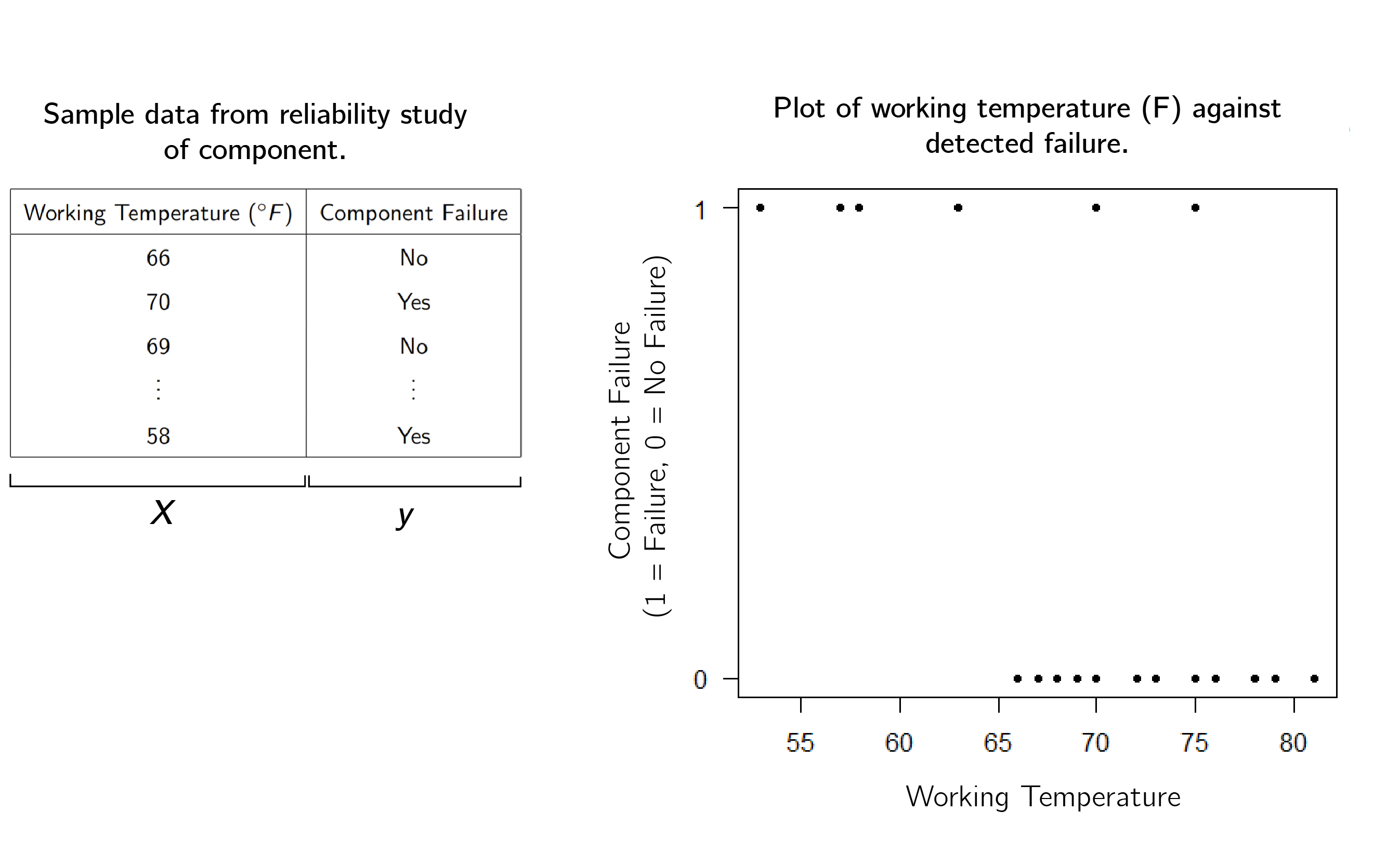
One method of performing binary classification is called Logistic Regression. The idea is to fit a curve to the data
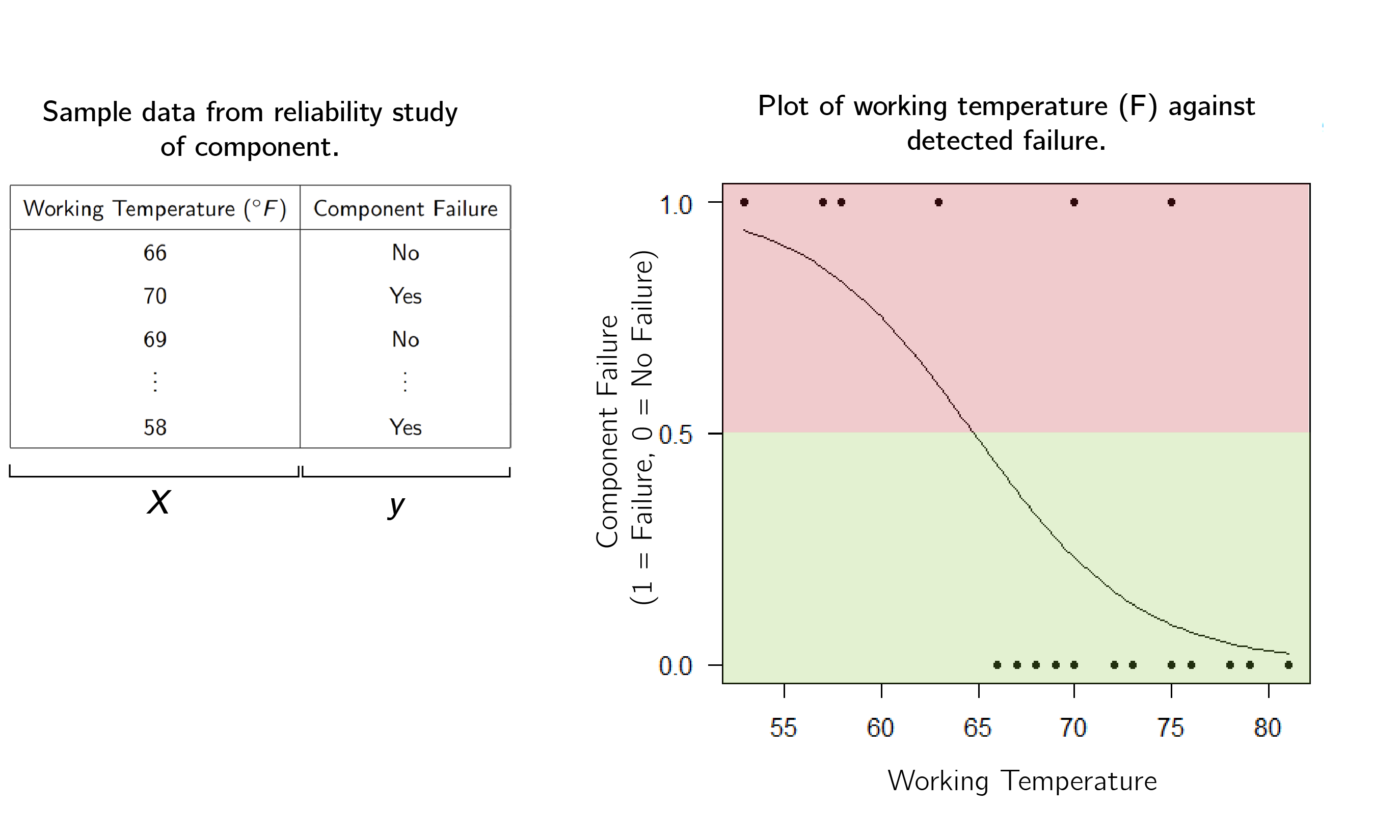
\[f(x) = \frac{1}{1+e^{-(\beta_0 + \beta_1 x)}}\]by calculating coefficients $\beta_0$ and $\beta_1$. Here, we used $(\beta_0,\beta_1) = (15.0429, -0.2321627).$ Where the curve is above one half (the red region) we would predict that the component will fail, and where the curve is below one half (the green region) we predict that the component will be alright.
The example we gave has one dimension (temperature) but we can generalise this concept to many dimensions. For a data matrix $\Bf X_{n\times p+1}$, we can fit instead fit a coefficient vector $\Bs{\beta} = (\beta_0,\dotsb, \beta_p)$. Then we obtain an estimator
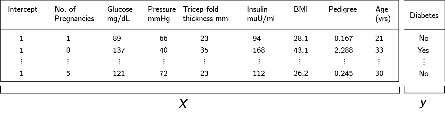
\[f(\mathbf{X}) = \frac{1}{1+e^{-\Bf X \Bs \beta}}\,.\]For example, consider the Pima Indians Diabetes dataset, which measures several predictors of diabetes, $(\mathbf X)$ and whether the test subject does have diabetes as the response $(\mathbf y)$.
However, in the case of many dimensions, we should be careful, because it is likely that not all of the predictors are relevant. Hence, we need to select for the most relevant features. To do this, let $\mathbf{w} \in \{0,1\}^{p+1}$ be a vector and $\Bf W = \mathrm{diag}(\Bf w)$. We call the matrix $\Bf W$ a binary mask, and consider instead
\[f(\mathbf{X}) = \frac{1}{1+e^{-\Bf X \Bf W \Bs \beta}}\,.\]Now, if the $i$-th entry $w_i$ of the binary mask $\mathbf w$ is $0$, then the $i$-th predictor $\beta_i$ in the regression coefficient vector $\Bs \beta$ will be multiplied by $0$, and have no effect on $f(\mathbf X)$. This way, the feature is dropped from the estimator.
\[\Bf X \Bf W \Bs \beta = \underbrace{\begin{bmatrix} 1 & \mathrm{preg}_0 & \cdots & \mathrm{age}_0 \\ \vdots & \vdots & \ddots & \vdots \\ 1 & \mathrm{preg}_p& \cdots & \mathrm{age}_p \\ \end{bmatrix} }_{X} \underbrace{\begin{bmatrix} w_0 & 0 & 0 \\ 0 & \ddots & 0 \\ 0 & 0 & w_p \\ \end{bmatrix} }_{W \text{ where } w_i \in \{0,1\}} \underbrace{\begin{bmatrix} \beta_0 \\ \vdots \\ \beta_p \\ \end{bmatrix} }_{\Bs \beta}\,.\]The process of selecting the relevant predictors for the model is also called model selection.
Fitting the Model
In order to perform inference with our estimator, we need two sets of parameters: some regression coefficients $\Bs \beta$, and a binary mask $\mathbf w$ for selecting our features. We are particularly interested with computing these parameters via Bayesian inference.
The main idea is to use Bayes’ Rule.
Definition (Bayes' Rule)
Suppose we want to estimate a parameter $\Bs \theta$, having observed data $\Bs x$. If we assume a \textit{prior} distribution $p(\Bs \theta)$, then we have $$ p(\Bs \theta \mid \Bf x) =\frac{p( \Bf x \mid \Bs \theta ) p(\Bs \theta)}{ \int p(\Bf x \mid \Bs \theta ) p(\Bs \theta) d\Bs \theta }\,. $$ We call $p(\Bs\theta \mid \mathbf x)$ the posterior density.
The idea is that, if we have some prior belief or knowledge about the location of our parameter $\Bs \theta$ within our parameter space, and then we observe some data, then we can use Bayes’ Rule to update our best guess of where $\Bs \theta$ lies.
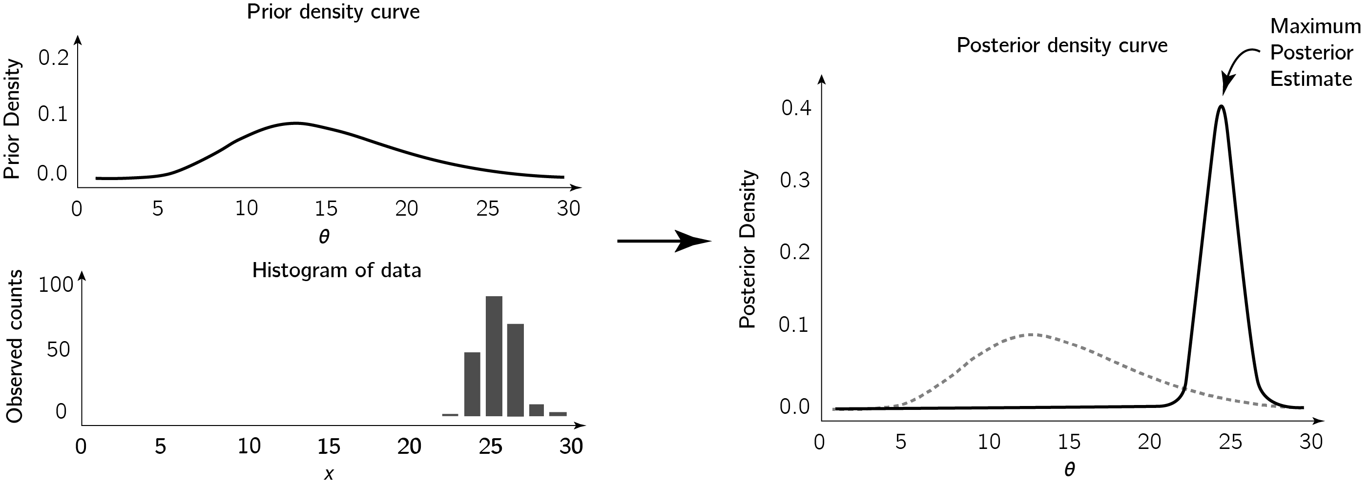
As shown in the figure, we might take the mode of the posterior density as our estimate for the parameter $\Bs \theta$. This esimtate is called the Maximium Posterior Estimate.
However, there is a big challenge. It is often extremely difficult to compute the integrals involved. For these reason, real world implementations of Bayesian inference revolves around methods of approximating the posterior. One such method is called variational Bayes.
For an arbitrary density $q(\theta)$, define the Kullback-Leiber ($\mathrm{KL}$) divergence to be
\[\mathrm{KL}(q(\Bs \theta),p(\Bs \theta \mid \Bf x)) = \int q(\Bs \theta) \log\left(\frac{q(\Bs \theta)}{p(\Bs \theta \mid \Bf x)}\right) d\Bs \theta \,.\]The idea of variational Bayes is to transform the integration problem into an optimisation problem, and approximate the posterior by finding densities $q(\Bs \theta)$ that minimise the $\mathrm{KL}$ divergence instead.
In particular, if we let $(\Bs \theta_1,\dotsb,\Bs \theta_M)$ be a partition of our parameter $\Bs \theta$, and assume that each partition is independent (called the mean-field approximation), we would have
\[q(\Bs \theta) = \prod_{i=1}^M q_i(\Bs \theta_i)\,,\]and then the optimal $q^*(\theta)$ for minimising $\mathrm{KL}$ would therefore be
\[\begin{equation} \label{eq:vb} q_i^*(\theta_i) \propto \exp\mathbb E_{-\theta_i}\log(p(\Bf x, \Bs \theta))\,. \end{equation}\]First approach: Use Variational Bayes
Now, we can define our problem. We want to create a predictive model for a logistic regression experiment with:
- Data matrix $\mathbf{X}$ with $p$ variables
- Binary response vector $\mathbf{y}$
- Regression coefficients $\boldsymbol{\beta} = (\beta_0, \ldots, \beta_p)$ with priors $\beta_j \sim \mathrm{Normal}(0, \sigma^2)$
- Model selection coefficients $\Gamma = (\gamma_0, \ldots, \gamma_p)$ with priors $\gamma_j \sim \mathrm{Bernoulli}(\rho)$
From the parameter space, we will partition $(\Bs \beta,\Gamma)$ into $(\Bs \beta, \gamma_0,\dotsb,\gamma_p)$. Using \ref{eq:vb}, we derive the following variational Bayes estimates for the parameter densities
\[\begin{aligned} q(\Bs \beta) &\propto \exp\left[ \mathcal{L}(\Bs \beta, \Bf X \Bf W , \Bf y) \right] \\ q(\gamma_j) &= \frac{\exp(\tau(\gamma_j))}{\exp(\tau(0))+\exp(\tau(1))} \end{aligned}\]where
\[\tau(\gamma_j) := (\Bf X^T \Bf y)_j \mu_j\gamma_j -1^T \log(1+ \exp(\Bf X_j \gamma_j \mu_j + \Bf X_{-j} \Bf W_{-j} \Bs\mu_{-j}) + \gamma_j \log{\left(\frac{\rho}{1-\rho}\right)}\]and
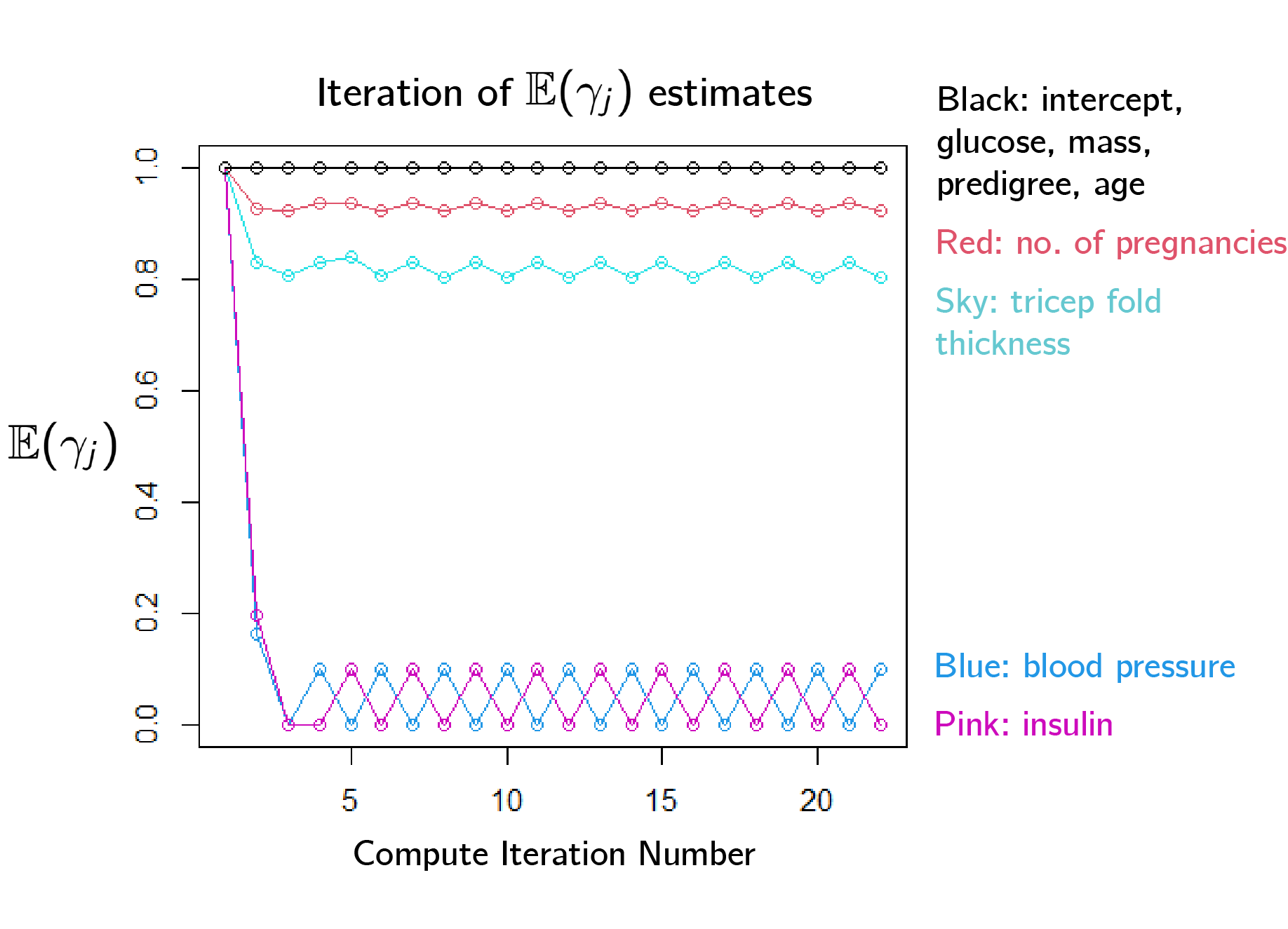
\[\mathcal{L}(\Bs \beta, \Bf X \Bf W , \Bf y) := \Bf y^T \Bf X \Bf W \Bs \beta - \Bf 1^T \log(\Bf 1 +\exp(\Bf X\Bf W \Bs \beta)) -\frac{1}{2\sigma^2}\| \Bs \beta \|^2\]However, when we tried to perform parameter estimation on the pima dataset with this system, we found that the model selection coefficients could not converge.
Second Approach: Use Reverse Collapsed Variational Bayes
In response, we alter our approach slightly. We perform variational Bayes estimates at both $\gamma_j =0$ and $\gamma_j = 1$ and then combine the data by integrating out $\Bs \beta$.
\[q(\gamma_j = k) \propto \int_{\mathbb{R}^p} \exp{ \left[ \mathcal{L}(\Bs \beta, \Bf Z , \Bf y) + k\log{\frac{\rho}{1-\rho}} \right]} d\Bs \beta \,.\]Again, this integral is difficult, so we approximate using the first order Laplace approximation $\Bs \beta \sim N( \widetilde{\Bs \beta} , \widetilde{\Bs \Sigma})$.
We get
\[q(\gamma_j = k) = \frac{|\Bs \Sigma_k|^{\frac12} \exp{\nu{(1)}} }{|\Bs\Sigma_1|^{\frac12}\exp{\nu{(1)}} + |\Bs\Sigma_0|^{\frac12}\exp{\nu{(0)}}}\]where $\Bs \Sigma_k$ is the covariance matrix of the $\Bs \beta$ Normal approximation at $\gamma_j = k$ and
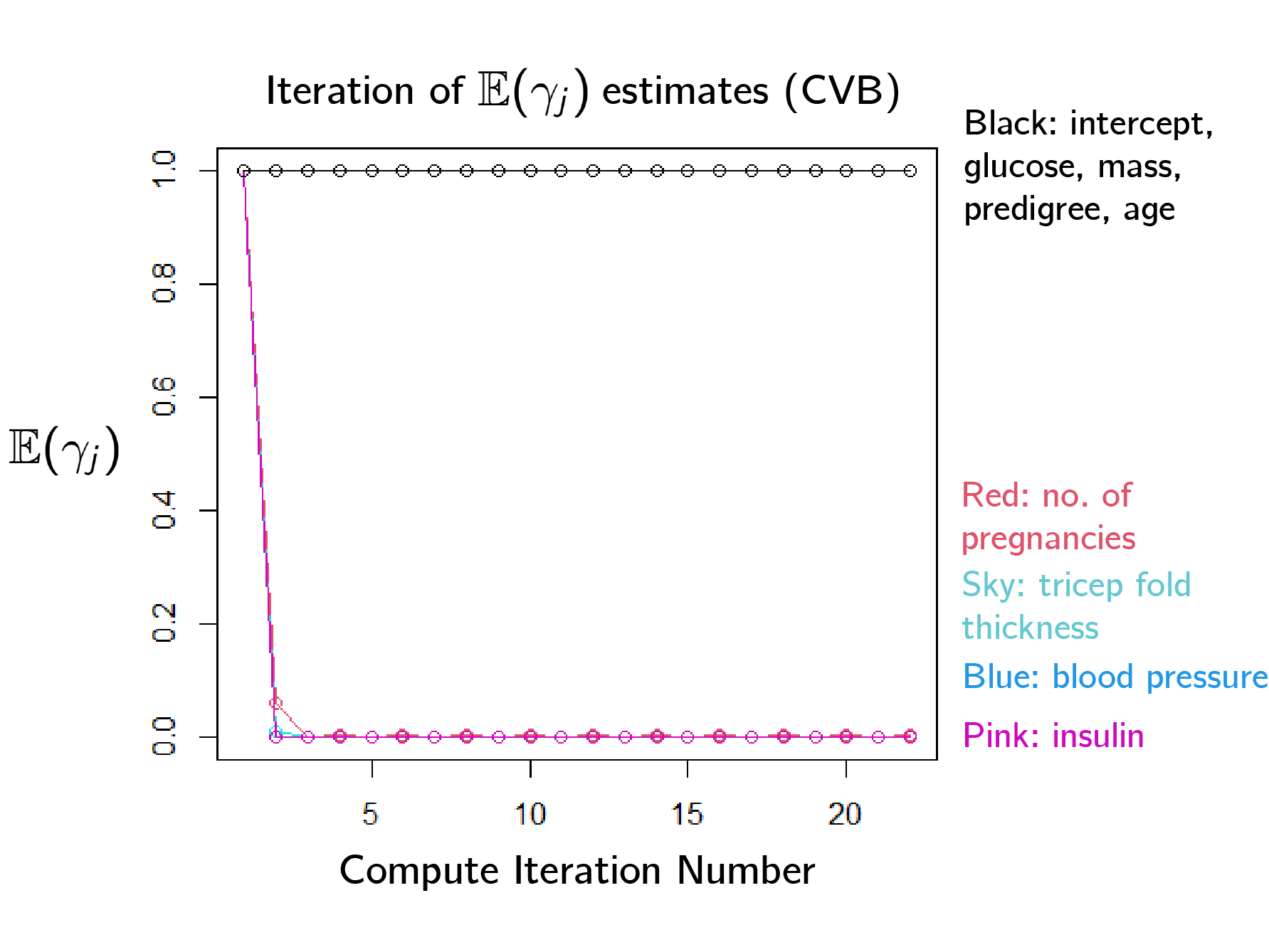
\[\begin{aligned} \nu(k) := \mathcal{L}(\Bs \beta, \Bf Z , \Bf y) - \frac12 \log{\det(-\Bf \Sigma_k)} + k\log\left(\frac{\rho}{ 1-\rho}\right) \,. \end{aligned}\]This new method was indeed able to converge, and quickly settle on the significant predictors.
Now, we can perform simultaneous model fitting and selection. For analysis of our results, see the full report here.